Recently, while studying GANs, I found that most of the current overview articles on GANs are from 2016 by Ian Goodfellow or from Professor Wang Feiyue of the Automation Institute. However, in the field of deep learning and GANs, progress is measured in months, and those two overviews feel a bit outdated.

Recently, I discovered a new overview paper on GANs that is over forty pages long, introducing various aspects of GANs. I have studied and organized my notes below. Much of the content in this article is summarized based on what I have learned, and any inaccuracies are welcome to be pointed out.

Additionally, this article references many blog materials, and links have been provided. If there is any infringement, please contact me for removal. The table of contents is as follows:

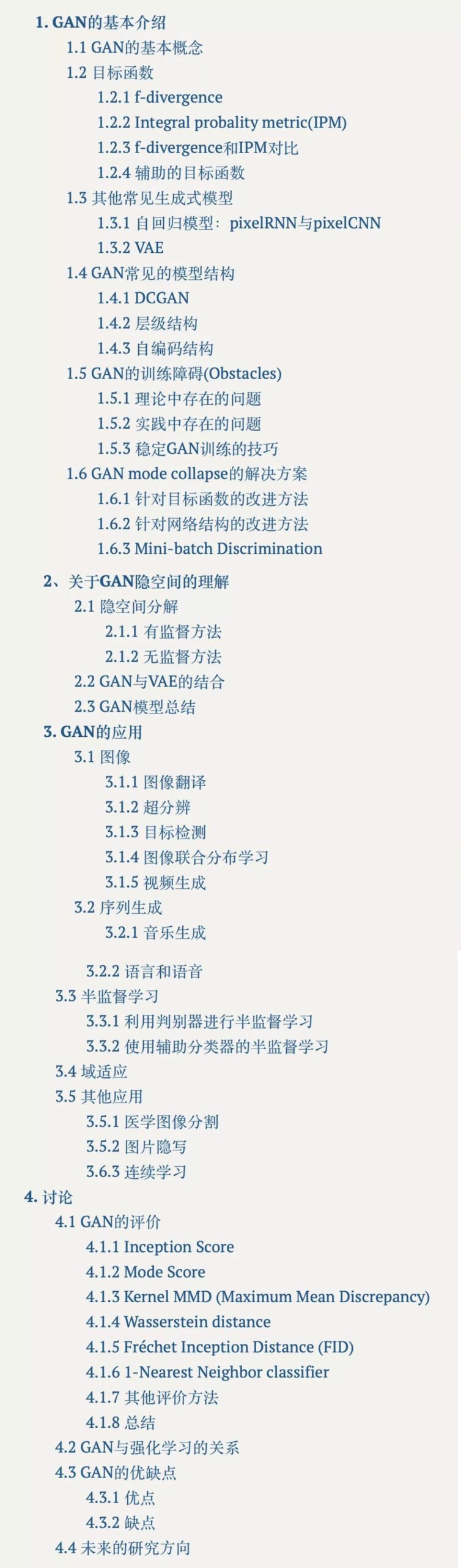
Basic Introduction to GAN

Generative Adversarial Networks (GAN) are an excellent generative model that has sparked many interesting applications in image generation. Compared to other generative models, GANs have two main characteristics:

1. They do not rely on any prior assumptions. Many traditional methods assume that data follows a certain distribution and then use maximum likelihood to estimate the data distribution.

2. The method of generating real-like samples is very simple. GAN generates real-like samples through the forward propagation of the generator, while traditional methods have very complex sampling methods. Interested readers can refer to Professor Zhou Zhihua’s book “Machine Learning” for an introduction to various sampling methods.

Next, we will elaborate on the above two points.

Basic Concepts of GAN

GAN (Generative Adversarial Networks) is, as the name suggests, a generative and adversarial network. More specifically, it learns a generative model of data distribution through adversarial methods.

The so-called adversarial refers to the mutual opposition between the generator network and the discriminator network. The generator network tries to generate realistic samples, while the discriminator network tries to determine whether the sample is real or generated. The schematic diagram is as follows:

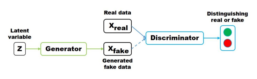
The latent variable z (usually random noise following a Gaussian distribution) generates Xfake through the generator, and the discriminator is responsible for determining whether the input data is the generated sample Xfake or the real sample Xreal. The optimization objective function is as follows:

For the discriminator D, this is a binary classification problem, and V(D,G) is a common cross-entropy loss in binary classification problems. For the generator G, in order to deceive D as much as possible, it needs to maximize the probability of the generated sample being classified by D, i.e., minimize log(1-D(G(z))). Note: The log(D(x)) term is independent of the generator G and can be ignored.

During actual training, the generator and discriminator are alternately trained, i.e., first train D, then train G, and continue this back and forth. It is worth noting that for the generator, its minimization is 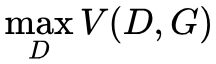, which minimizes the maximum of V(D,G).

In order to ensure that V(D,G) achieves the maximum, we usually train the discriminator for k iterations and then iterate once for the generator (although in practice, k is usually taken as 1). When the generator G is fixed, we can derive V(D,G) to find the optimal discriminator D*(x):

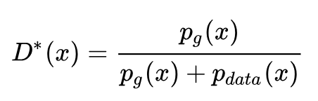
Substituting the optimal discriminator into the above objective function allows us to further find that under the optimal discriminator, the generator’s objective function is equivalent to optimizing the JS divergence (JSD, Jensen-Shannon Divergence) between Pdata(x) and Pg(x).

It can be proven that when both G and D have sufficient capacity, the model will converge, and both will reach Nash equilibrium. At this point, Pdata(x)=Pg(x), and the discriminator will predict probabilities of 1/2 for samples drawn from either Pdata(x) or Pg(x), meaning the generated samples and real samples have become indistinguishable.

Objective Function

Earlier, we mentioned that the objective function of GAN is to minimize the JS divergence between two distributions. In fact, there are many ways to measure the distance between two distributions; JS divergence is just one of them. If we define different distance metrics, we can obtain different objective functions. Many improvements to GAN training stability, such as EBGAN, LSGAN, etc., define different distance metrics between distributions.

f-divergence

f-divergence defines the distance between two distributions using the following formula:

In the above formula, f is a convex function, and f(1)=0. By adopting different f functions (Generators), we can obtain different optimization objectives. Specifically:

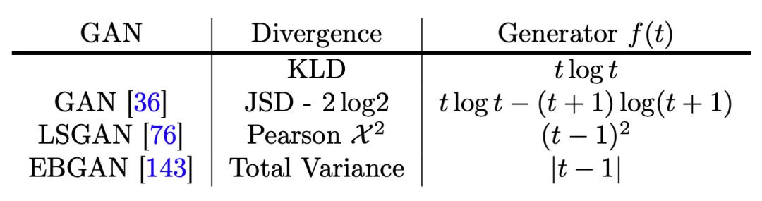
It is worth noting that this divergence measure is not symmetric, i.e., Df(Pdata||Pg) and Df(Pg||Pdata) are not equal.

LSGAN

As mentioned above, LSGAN is a special case when 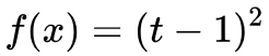in f-divergence. Specifically, the Loss of LSGAN is as follows:

In the original work, a=c=1, b=0. LSGAN has two main advantages:

• Stable training: It addresses the gradient saturation problem in traditional GAN training processes.

• Improved generation quality: It achieves this by penalizing generated samples that are far from the discriminator’s decision boundary.

For the first point, stable training, we can first look at a diagram:

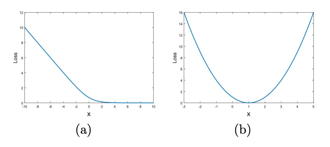
The left side of the diagram shows the correlation between input and output when traditional GAN uses sigmoid cross-entropy as loss. The right side shows the correlation when LSGAN uses least squares loss. As we can see, in the left diagram, when the input is large, the gradient is 0, indicating that the input to the cross-entropy loss easily experiences gradient saturation. The right side with least squares loss does not have this issue.

For the second point, improving generation quality. This is also explained in detail in the original text. Specifically: for some samples that the discriminator classifies correctly, their gradient does not contribute. However, is it true that samples classified correctly by the discriminator are necessarily very close to the real data distribution? Clearly, not necessarily.

Consider the following ideal situation: a well-trained GAN has a real data distribution Pdata and a generated data distribution Pg that completely overlap, with the discriminator’s decision boundary passing through real data points. Therefore, we can use the distance of sample points from the decision boundary to measure the quality of generated samples; the closer the sample is to the decision boundary, the better the GAN is trained.

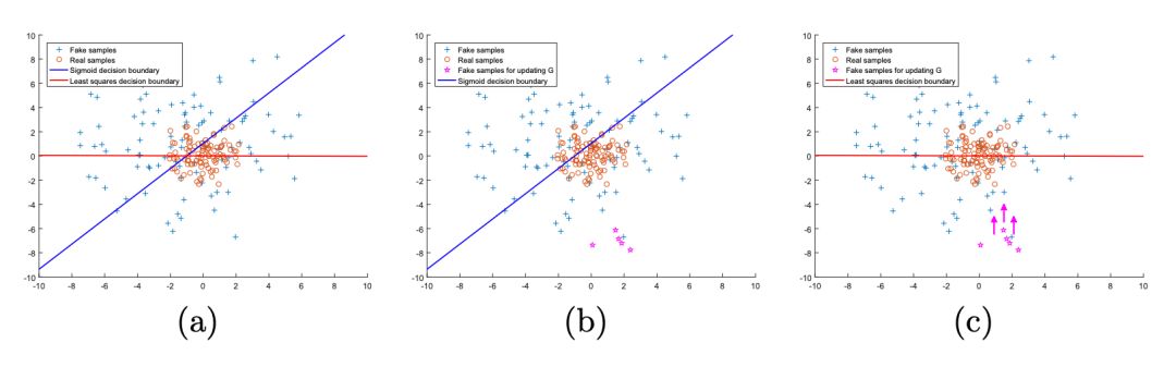
In diagram b above, some points that are far from the decision boundary, although classified correctly, are not good generated samples. Traditional GANs usually ignore them. However, for LSGAN, due to the use of least squares loss, it calculates the distance from the decision boundary to the sample points, as shown in diagram c, which can “pull” back points that are far from the decision boundary, i.e., points that are far from real data.

Integral Probability Metric (IPM)

IPM defines a family of evaluation functions f, which are used to measure the distance between any two distributions. In a compact space 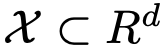, define P(x) as the probability measure at x. The IPM between two distributions Pdata and Pg can be defined as follows:

Similar to f-divergence, different functions f can also define a series of different optimization objectives. Typical examples include WGAN, Fisher GAN, etc. Below is a brief introduction to WGAN.

WGAN

WGAN proposes a completely new distance metric—the Earth Mover’s Distance (EM), also known as Wasserstein Distance. For an introduction to Wasserstein Distance, refer to: Understanding Wasserstein Distance [1].

The specific definition of Wasserstein distance is as follows:

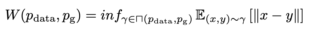
⊓(Pdata,Pg) represents a set of joint distributions, where any distribution γ in this joint distribution has marginal distributions that are Pdata(x) and Pg(x).

Intuitively, the probability distribution function (PDF) can be understood as the mass of the random variable at each point, so W(Pdata,Pg) represents the minimum amount of work required to move the probability distribution Pdata(x) to Pg(x).

WGAN can also be explained using optimal transport theory, where the generator of WGAN is equivalent to solving the optimal transport mapping, and the discriminator is equivalent to calculating the Wasserstein distance, i.e., the total cost of optimal transport [4]. The theoretical derivation and explanation of WGAN are quite complex, but the code implementation is very simple. Specifically [3]:

• The last layer of the discriminator removes the sigmoid function.

• The loss of the generator and discriminator is not taken as log.

• After updating the parameters of the discriminator, truncate their absolute values to not exceed a fixed constant c.

The third point mentioned above, in a later work of WGAN called WGAN-GP, replaced gradient clipping with gradient penalty.

Comparison of f-divergence and IPM

f-divergence has two problems: first, as the dimensionality 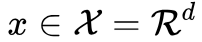of the data space increases, f-divergence becomes very difficult to calculate. Second, the support sets of the two distributions [3] are usually not aligned, which will cause the divergence value to approach infinity.

IPM, on the other hand, is not affected by the dimensionality of the data and consistently converges to the distance between the two distributions Pdata and Pg. Moreover, even when the support sets of the two distributions do not overlap, it will not diverge.

Auxiliary Objective Functions

In many applications of GAN, additional losses are used to stabilize training or achieve other goals. For example, in image translation, image restoration, and super-resolution, the generator may incorporate target images as supervisory information. EBGAN uses the GAN discriminator as an energy function, incorporating reconstruction error into the discriminator. CGAN uses class label information as supervisory information.

Other Common Generative Models

Autoregressive Models: PixelRNN and PixelCNN

Autoregressive models explicitly model the probability distribution Pdata(x) of image data and optimize the model using maximum likelihood estimation. Specifically:

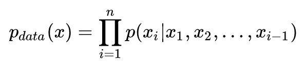
The above formula is easy to understand; given x1,x2,…,xi-1, the product of all p(xi) probabilities represents the distribution of image data. If RNN is used to model the above relationship, it is PixelRNN. If CNN is used, it is PixelCNN. Specifically [5]:

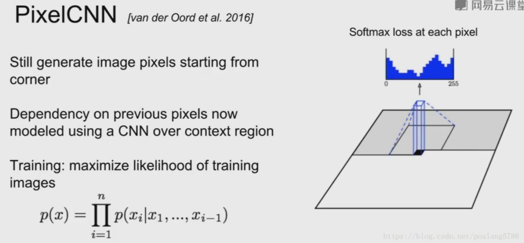
Clearly, both PixelCNN and PixelRNN generate pixel values one by one, making the process very slow. WaveNet, which has become popular in the speech domain, is a typical autoregressive model.

VAE

PixelCNN/RNN defines a manageable density function that we can directly optimize the likelihood of the training data; for Variational Autoencoders (VAEs), we define a more complex density function by modeling it with additional latent variables z. The principle of VAE is as follows [6]:

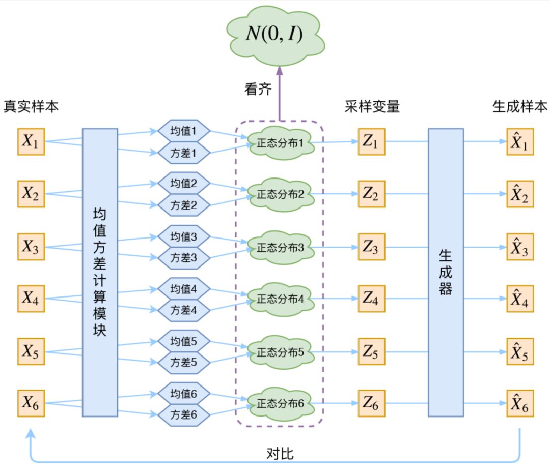
In VAE, real samples X pass through a neural network to compute mean and variance (assuming the latent variable follows a normal distribution), then samples the latent variable Z and reconstructs. Both VAE and GAN learn the mapping from latent variable z to the real data distribution. However, unlike GAN:

1. GAN’s approach is more straightforward, using a discriminator to measure the distance between the distribution generated by the distribution transformation module (i.e., generator) and the real data distribution.

2. VAE is not as intuitive; VAE achieves the distribution transformation mapping X=G(z) by constraining the latent variable z to follow a standard normal distribution and reconstructing the data.

Comparison of Generative Models

1. Autoregressive models generate data by explicitly modeling the probability distribution;

2. Both VAE and GAN are: assuming that the latent variable z follows a certain distribution and learning a mapping X=G(z) to realize the transformation between the latent variable distribution z and the real data distribution Pdata(x);

3. GAN uses a discriminator to measure the quality of the mapping X=G(z), while VAE measures it through the KL divergence between the latent variable z and the standard normal distribution and the reconstruction error.

Common GAN Model Structures

DCGAN

DCGAN proposes using CNN structures to stabilize GAN training and employs the following tricks:

• Batch Normalization

• Using Transpose Convolution for upsampling

• Using Leaky ReLU as the activation function

These tricks significantly aid in stabilizing GAN training, and can be used judiciously when designing GAN networks.

Hierarchical Structures

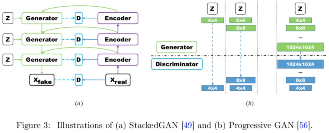
GAN has faced many issues in generating high-resolution images. Hierarchical GANs generate images in a stepwise, staged manner to gradually increase the resolution. Typical models using multiple GANs include StackGAN and GoGAN. The structures of StackGAN and ProgressiveGAN are as follows:

Autoencoder Structures

In classic GAN structures, the discriminator network is usually treated as a probabilistic model used to distinguish between real/generated samples. In autoencoder structures, the discriminator (using AE as the discriminator) is often treated as an energy function. For samples that are close to the data manifold space, their energy is low, and vice versa. With this distance metric, the discriminator can guide the learning of the generator.

Why can AE be used as a discriminator and treated as an energy function to measure the distance of generated samples from the data manifold space? First, let’s look at the loss of AE:

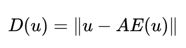
The loss of AE is a reconstruction error. When using AE as a discriminator, if the input is a real sample, its reconstruction error will be small. If the input is a generated sample, its reconstruction error will be large. This is because it is difficult for AE to learn a compressed representation of an image for generated samples (i.e., generated samples are far from the data manifold space). Therefore, the reconstruction error of VAE is a reasonable measure of the distance between Pdata and Pg.

Typical autoencoder structures of GAN include: BEGAN, EBGAN, MGAN, etc.

Training Obstacles for GAN

Theoretical Issues

Classic GAN’s discriminator has two types of loss:

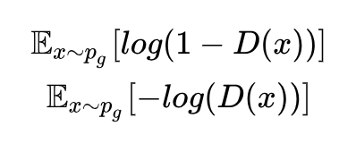
Using the first formula above as loss: when the discriminator reaches optimality, it is equivalent to minimizing the JS divergence between the generated distribution and the real distribution. Due to the random generated distribution’s difficulty in having a non-negligible overlap with the real distribution and the sudden change characteristics of JS divergence, the generator faces the problem of vanishing gradients.

Using the second formula above as loss: under the optimal discriminator, it is equivalent to minimizing the KL divergence between the generated distribution and the real distribution while maximizing its JS divergence, which is contradictory, leading to unstable gradients. Moreover, the asymmetry of KL divergence causes the generator to prefer to lose diversity rather than accuracy, leading to the mode collapse phenomenon [7].

Practical Issues

GAN faces two issues in practice:

First, although Ian Goodfellow, the proposer of GAN, theoretically proved that GAN can reach Nash equilibrium, in actual implementation, we optimize in parameter space rather than function space, which leads to theoretical guarantees not being valid in practice.

Second, the optimization objective of GAN is a min-max problem, i.e., 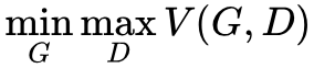. This means that when optimizing the generator, we minimize 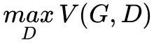. However, we iterate optimization, and to ensure that V(G,D) is maximized requires many iterations, leading to long training times.

If we only iterate once for the discriminator and then once for the generator, continuously cycling, the original min-max problem can easily turn into a max-min problem (maxmin), which is not the same, i.e.:

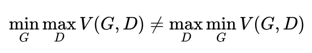
If it changes to a min-max problem, then the iterations would be like this: the generator first generates some samples, then the discriminator gives incorrect judgment results and punishes the generator, which causes the generator to adjust the generated probability distribution. However, this often leads to the generator becoming “lazy”, only generating some simple, repetitive samples, lacking diversity, also known as mode collapse.

Techniques to Stabilize GAN Training

As mentioned above, GAN has three major issues in theory and practice, leading to very unstable training processes and the mode collapse problem. To improve the above situation, the following techniques can be used to stabilize training:

Feature Matching: This method is straightforward; it replaces the output of the original GAN Loss with the features from a certain layer of the discriminator. That is, minimize: the distance between the features obtained from the discriminator for generated images and real images.

Label Smoothing: In GAN training, labels are either 0 or 1, which causes the confidence predicted by the discriminator to tend to higher values. Using label smoothing can alleviate this issue. Specifically, replace label 1 with a random number between 0.8 and 1.0.

Spectral Normalization: WGAN and Improved WGAN impose Lipschitz conditions to constrain the optimization process. Spectral normalization applies Lipschitz constraints to every layer of the discriminator, but is computationally more efficient than Improved WGAN.

PatchGAN: To be accurate, PatchGAN is not used for stabilizing training, but this technique is widely used in image translation. PatchGAN acts as a discriminator for each small patch of the image, allowing the generator to produce sharper, clearer edges.

The specific practice is as follows: assume a 256×256 image is input to the discriminator, the output is a 4×4 confidence map, where each pixel value in the confidence map represents the confidence that the current patch is a real image, which is PatchGAN. The current image patch size is the size of the receptive field, and finally, the losses of all patches are averaged to form the final loss.

Solutions to Mode Collapse

Improvement Methods for Objective Functions

To avoid the mode jumping problems caused by optimizing maxmin mentioned earlier, UnrolledGAN modifies the generator loss to address this. Specifically, UnrolledGAN updates the generator k times when updating the generator, referencing the loss not from one instance but from the loss of the discriminator in the subsequent k iterations.

Note that in the subsequent k iterations, the discriminator does not update its parameters; it only calculates the loss for updating the generator. This method allows the generator to consider the changes in the discriminator over the next k iterations, avoiding the mode collapse problem caused by switching between different modes. It is crucial to distinguish this from iterating generator k times and then iterating the discriminator once [8].

DRAGAN introduces a no-regret algorithm from game theory, modifying its loss to address the mode collapse problem [9]. The previously mentioned EBGAN adds the VAE reconstruction error to resolve mode collapse.

Improvement Methods for Network Structures

Multi-Agent Diverse GAN (MAD-GAN) employs multiple generators and one discriminator to ensure the diversity of generated samples. The specific structure is as follows:

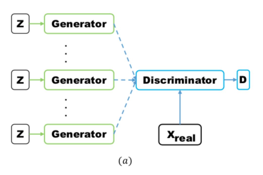
Compared to ordinary GAN, it adds several generators, and when designing the loss, a regularization term is included. The regularization term uses cosine distance to penalize the consistency of samples generated by the three generators.

MRGAN adds a discriminator to penalize the mode collapse problem of generated samples. The specific structure is as follows:

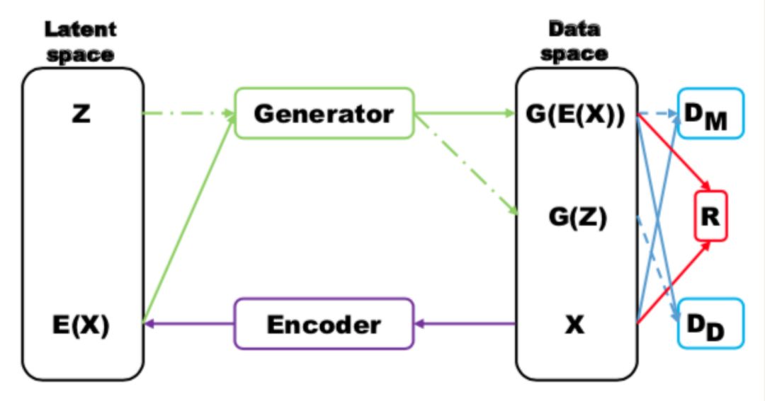
The input sample x is encoded into the latent variable E(x) through an Encoder, and then the latent variable is reconstructed by the Generator. During training, there are three losses. DM and R (reconstruction error) guide the generation of real-like samples. DD is used to discern whether E(x) and the samples generated by z are fake samples, thus this discriminator mainly determines whether the generated samples exhibit diversity, i.e., whether mode collapse occurs.

Mini-Batch Discrimination

Mini-batch discrimination establishes a mini-batch layer in the middle of the discriminator to compute statistics based on L1 distance, allowing the discriminator to utilize this information to discern which samples lack diversity. For the generator, it should strive to generate samples with diversity.

Understanding the Latent Space of GAN

The latent space is a compressed representation space of the data. Generally, it is unrealistic to modify images directly in data space because image attributes lie in the manifold of high-dimensional space. However, in the latent space, since each latent variable represents a specific attribute, this is feasible.

In this section, we will explore how GAN handles the latent space and its attributes, and also discuss how variational methods can be integrated into the GAN framework.

Latent Space Decomposition

The input latent variable z of GAN is unstructured, and we do not know what each bit of the latent variable controls. Therefore, some scholars have proposed decomposing the latent variable into a conditional variable c and a standard input latent variable z. This includes both supervised and unsupervised methods.

Supervised Methods

Typical supervised methods include CGAN and ACGAN.

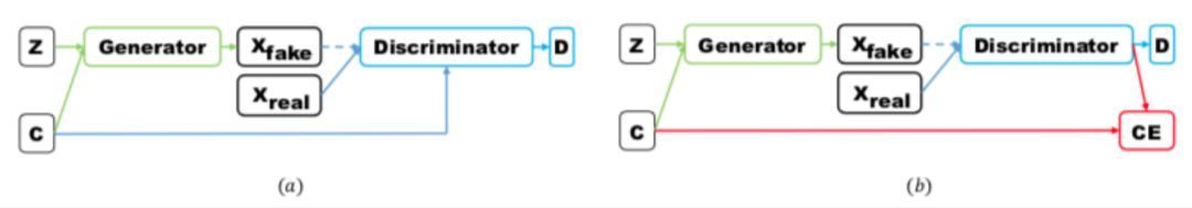
CGAN takes random noise z and class labels c as inputs to the generator, while the discriminator takes the generated samples/real samples along with the class labels as inputs. This learns the correlation between labels and images.

ACGAN takes random noise z and class labels c as inputs to the generator, while the discriminator takes the generated samples/real samples as inputs and also regresses the class labels of the images. This learns the correlation between labels and images. The structures of the two are as follows (left is CGAN, right is ACGAN):

Unsupervised Methods

In contrast to supervised methods, unsupervised methods do not use any label information. Therefore, unsupervised methods need to decouple the latent space to obtain meaningful feature representations.

InfoGAN decomposes the input noise into latent variable z and conditional variable c (during training, the conditional variable c is sampled from a uniform distribution) and sends both to the generator. During training, it maximizes the mutual information I(c;G(z,c)) to achieve variable decoupling (I(c;G(z,c)) mutual information indicates how much information c contains about G(z,c)).

The model structure is basically the same as CGAN, except that the loss includes an additional term for maximizing mutual information. Specifically: [10]:

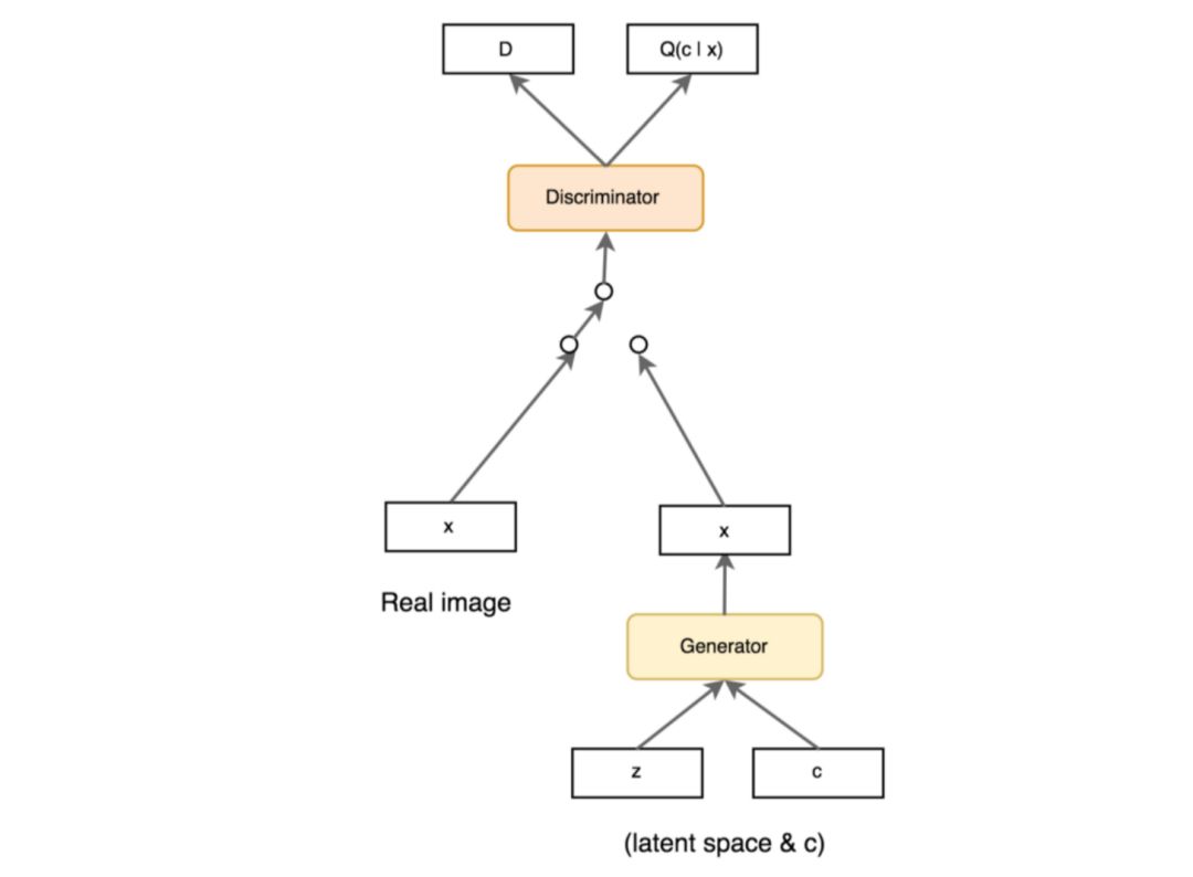
From the above analysis, it can be seen that InfoGAN only achieves information decoupling, but we cannot control what each value of the conditional variable c specifically means.

Thus, ss-InfoGAN appears, which adopts a semi-supervised learning method, dividing the conditional variable c into two parts, 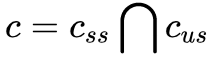. Css learns using labels like CGAN, while Cus learns like InfoGAN.

Combining GAN with VAE

GAN can generate clearer images compared to VAE, but it is prone to mode collapse issues. VAE, on the other hand, encourages reconstruction of all samples, thus avoiding mode collapse problems.

A typical work combining the two is VAEGAN, which has a structure similar to the previously mentioned MRGAN, as follows:

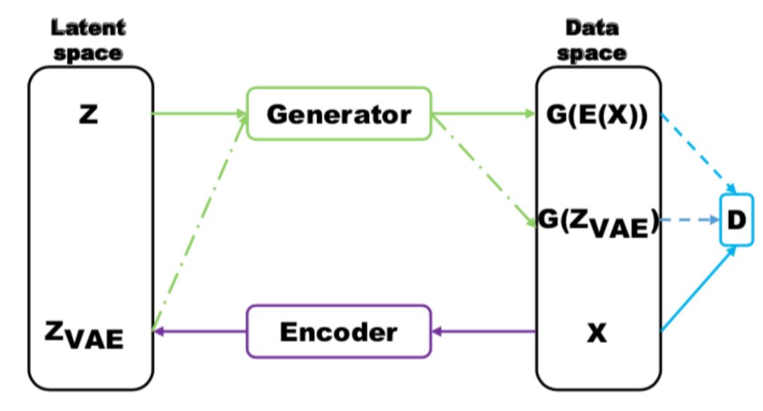
The loss of the above model includes three parts: the reconstruction error of the features from a certain layer of the discriminator, the VAE loss, and the GAN loss.

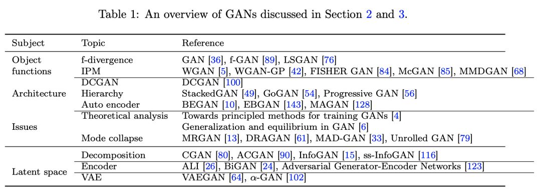
Summary of GAN Models

The previous two sections introduced various GAN models, most of which are designed around two common issues of GAN: mode collapse and training collapse. The table below summarizes these models, and readers can refer to this table for review:

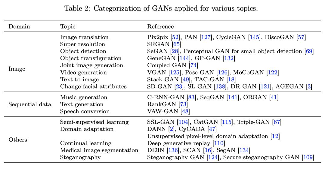
Applications of GAN

Since GAN can generate real-like samples without explicitly modeling any data distribution, GAN has widespread applications in images, text, speech, and many other fields. The table below summarizes GAN applications in various domains, which will be introduced in subsequent sections.

Images

Image Translation

Image translation refers to the conversion from one (source domain) image to another (target domain) image. It can be likened to machine translation, where one language is converted into another. In the translation process, the content of the source domain image remains unchanged, but the style or other attributes change to that of the target domain.

Paired Two-Domain Data

A typical example of paired image translation is pix2pix, which uses paired data to train a conditional GAN. The loss includes both GAN loss and pixel-wise difference loss. PAN uses pixel-wise difference on feature maps as perceptual loss instead of pixel-wise difference on images to generate images that are more visually similar to the source domain.

Unpaired Two-Domain Data

For image translation problems without paired training data, a typical example is CycleGAN. CycleGAN uses two pairs of GANs, converting source domain data to the target domain through one GAN network, and then converting target domain data back to the source domain through another GAN network. The data converted back is paired with the source domain data, forming supervisory information.

Super-resolution

SRGAN uses GAN and perceptual loss to generate detail-rich images. Perceptual loss focuses on the error of intermediate feature layers rather than pixel-wise error of the output result, avoiding the problem of generated high-resolution images lacking texture detail information.

Object Detection

Thanks to GAN’s application in super-resolution, for small object detection problems, GAN can generate high-resolution images of small objects to improve object detection accuracy.

Image Joint Distribution Learning

Most GANs learn the data distribution of a single domain, while CoupledGAN proposes a network with partially shared weights to learn the joint distribution of images across multiple domains using unsupervised methods. The specific structure is as follows [11]:

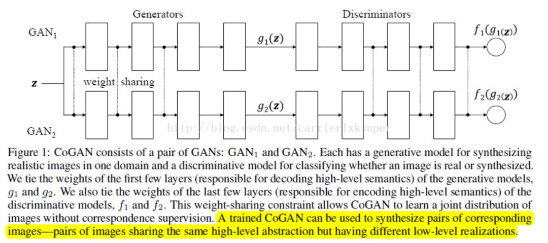
As shown in the figure above, CoupledGAN uses two GAN networks. The front half of the generator shares weights to encode the common high-level information of two domains, while the back half does not share weights to encode the data of each respective domain. The front half of the discriminator does not share weights, while the back half is used to extract high-level features and share weights between the two. For the trained network, inputting random noise generates two images from different domains.

It is worth noting that the above model learns the joint distribution P(x,y); if two separate GANs are trained separately, they will learn the marginal distributions P(x) and P(y). Typically, P(x,y)≠P(x)·P(y).

Video Generation

Typically, videos consist of relatively stationary backgrounds and moving foregrounds. VideoGAN uses a two-stage generator, where a 3D CNN generator generates moving foregrounds, and a 2D CNN generator generates stationary backgrounds.

Pose GAN uses VAE and GAN to generate videos. First, VAE combines the pose features of the current frame and past frames to predict the motion information of the next frame, and then the 3D CNN uses the motion information to generate subsequent video frames.

Motion and Content GAN (MoCoGAN) separates the motion and content parts in the latent space, using RNN to model the motion part.

Sequence Generation

Compared to GAN’s applications in the image domain, its applications in text and speech domains are fewer. The main reasons are twofold:

1. GAN uses the BP algorithm during optimization, which cannot directly jump to target values for discrete data like text and speech, and can only approach the target step by step based on gradients.

2. For sequence generation problems, for each generated word, we need to judge whether the sequence is reasonable, but the discriminator in GAN cannot do this. Unless we set a discriminator for each step, which is clearly unreasonable.

To address the above issues, policy gradient descent from reinforcement learning has been introduced into GAN for sequence generation problems.

Music Generation

RNN-GAN uses LSTM as both the generator and discriminator to directly generate an entire audio sequence. However, as mentioned above, treating music as including lyrics and notes, directly using GAN for this discrete data generation problem poses many issues, especially generating data lacking local consistency.

In contrast, SeqGAN uses the generator’s output as the strategy of an agent, and the output of the discriminator as the reward, using policy gradient descent to train the model. ORGAN builds upon SeqGAN, setting a specific objective function for specific goals.

Language and Speech

VAW-GAN (Variational Autoencoding Wasserstein GAN) combines VAE and WGAN to implement a speech conversion system. The encoder encodes the content of the speech signal, while the decoder is used to reconstruct the timbre. Due to VAE’s tendency to produce overly smooth results, WGAN is used here to generate clearer speech signals.

Semi-Supervised Learning

Obtaining labels for image data requires extensive manual annotation, a time-consuming and labor-intensive process.

Using Discriminator for Semi-Supervised Learning

The semi-supervised learning method based on GAN [12] proposes a method that utilizes unlabeled data. The implementation method is essentially the same as the original GAN, with the specific framework as follows [13]:

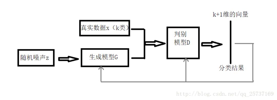
Compared to the original GAN, the main difference is that the discriminator outputs K+1 category information (the generated samples are the K+1 category). For the discriminator, its loss includes two parts: one is the supervised learning loss (which only needs to judge whether the sample is real or fake), and the other is the unsupervised learning loss (which judges the sample category). The generator only needs to generate realistic samples as much as possible. After training is complete, the discriminator can serve as a classification model.

From an intuitive perspective, the generated samples primarily assist the classifier in learning where the real data space is.

Using Auxiliary Classifiers for Semi-Supervised Learning

The model utilizing the discriminator for semi-supervised learning mentioned above has a problem. The discriminator has to learn to distinguish between positive and negative samples while also learning to predict labels. The two objectives are inconsistent and can easily lead to neither achieving optimal performance. An intuitive idea is to separate the prediction of labels from distinguishing positive and negative samples. Triple-GAN does just that [14]:

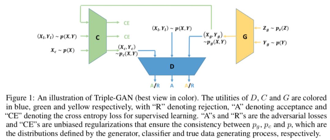
(Xg,Yg)~pg(X,Y), (Xl,Yl)~p(X,Y), (Xc,Yc)~pc(X,Y) represent generated data, labeled data, and unlabeled data respectively. CE represents cross-entropy loss.

Domain Adaptation

Domain adaptation is a concept in transfer learning. In simple terms, we define the source data domain distribution as Ds(x,y) and the target data domain distribution as DT(x,y). We have many labels for source domain data, but none for target domain data. We hope to learn a model that generalizes well in the target domain using the labeled data from the source domain and the unlabeled data from the target domain. The “transfer” in transfer learning refers to the transfer of the source domain data distribution to the target domain data distribution.

When GAN is applied to transfer learning, the core idea is to use the generator to convert the features of the source domain data into those of the target domain, while the discriminator tries to distinguish between real data and generated data features. Below are two examples of applying GAN to transfer learning, DANN and ARDA:

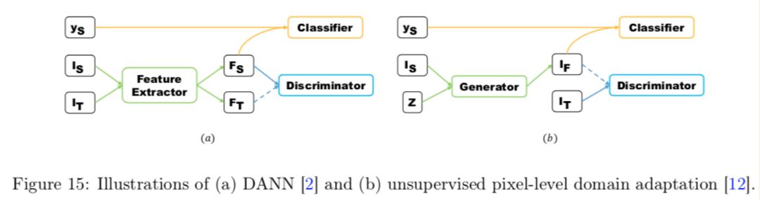
Taking DANN as an example, Is and It represent the source domain data and target domain data, respectively, while ys represents the labels of the source domain data. Fs and Ft represent the features of the source and target domains. In DANN, the generator is used to extract features and make the extracted features difficult for the discriminator to distinguish whether they are from the source domain or target domain data features.

In the field of person re-identification, many CycleGAN-based transfer learning applications have been used for data augmentation. One difficulty in the person re-identification problem is the significant differences in environments and angles of individuals captured by different cameras, leading to a large domain gap.

Therefore, it might be considered to use GAN to generate data under different camera settings for data augmentation.[15] proposed a CycleGAN method for data augmentation. The specific model structure is as follows:

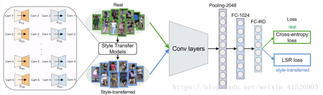
For each pair of cameras, a CycleGAN is trained, allowing the transformation of data from one camera to another while keeping the content (individual) unchanged.

Other Applications

GAN has numerous variants and applications, including in some non-machine learning fields. Below are a few examples:

Medical Image Segmentation

[16] proposed a segmentor-critic structure for segmenting medical images. The segmentor is similar to the generator in GAN, used to generate segmentation images, while the critic maximizes the distance between the generated segmentation images and the ground truth. Additionally, DI2IN uses GAN for segmenting 3D CT images, and SCAN uses GAN for segmenting X-ray images.

Image Steganography

Steganography refers to hiding secret information within a non-secret container, such as an image. Steganalysis is then used to determine whether the container contains secret information. Some studies have attempted to use the GAN generator to generate images with hidden information, while the discriminator has two roles: one to determine whether the image is real and the other to determine whether the image contains secret information [17].

Continual Learning

The goal of continual learning is to solve multiple tasks while continuously accumulating new knowledge. A prominent issue in continual learning is “knowledge forgetting.” [18] proposed using the GAN generator as a scholars model, where the generator continually trains using past knowledge, and the solver provides answers to avoid the “knowledge forgetting” problem.

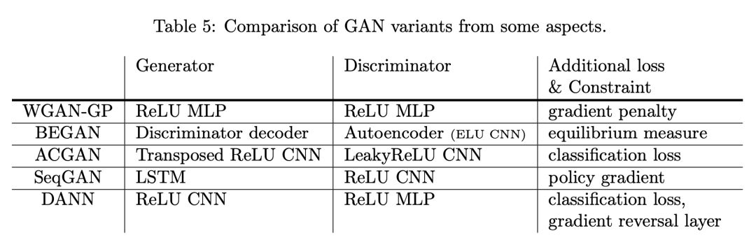
Discussion

In the first two parts, we discussed GAN and its variants, while the third part discussed the applications of GAN. The table below summarizes some well-known GAN model structures and the additional constraints applied.

The previous discussions focused on the micro-level of GAN. Next, we will take a macro perspective to discuss GAN.

Evaluation of GAN

There are various evaluation methods for GAN, and existing example-based methods (as the name suggests, evaluate based on sample level) extract features from generated samples and real samples, then measure distances in feature space. The specific framework is as follows:

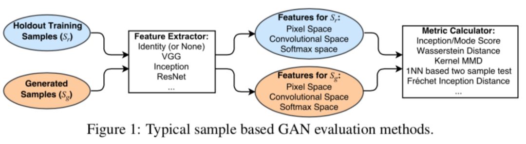
Regarding the symbols in this section, the following relationships apply:

Pg represents the distribution of generated data, Pr represents the distribution of real data, E represents the mathematical expectation, x represents input samples, x~Pg represents samples drawn from generated data, x~Pr represents samples drawn from real data. y represents sample labels, and M represents the classification network, typically choosing the Inception network.

Below, we will introduce common evaluation metrics one by one.

Inception Score

For a well-trained GAN on ImageNet, when the generated samples are tested with the Inception network, the resulting classification probabilities should exhibit the following characteristics:

1. For images of the same category, the output probability distribution should converge towards a pulse distribution, ensuring the accuracy of generated samples.

2. For all categories, the output probability distribution should converge towards a uniform distribution, preventing issues like mode collapsing and ensuring the diversity of generated samples.

Thus, the following metric can be designed:

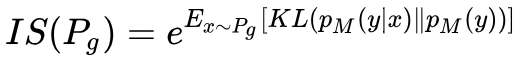
Based on the previous analysis, if it is a well-trained GAN, pM(y|x) approaches a pulse distribution, and pM(y) approaches a uniform distribution. The KL divergence between the two will be large, leading to a high Inception Score. Actual experiments show that Inception Score aligns well with human subjective judgments. The calculation of IS does not use real data, and its specific value depends on the choice of model M.

Characteristics: It can measure the diversity and accuracy of generated samples to some extent, but cannot detect overfitting. Mode Score is similarly limited and is not recommended for datasets that differ significantly from ImageNet.

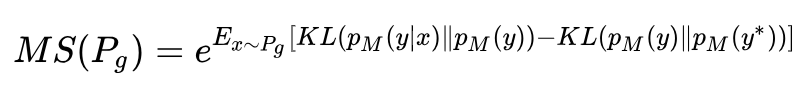
Mode Score

Mode Score is an improved version of Inception Score, adding a measure of similarity between the predicted probability distributions of generated and real samples. The specific formula is as follows:

Kernel MMD

The calculation formula is as follows:

For calculating the Kernel MMD value, a kernel function k must first be selected, mapping the samples to the Reproducing Kernel Hilbert Space (RKHS). RKHS has many advantages over Euclidean space and is complete for calculating inner products of functions.

Expanding the above formula yields the following calculation formula:

The smaller the MMD value, the closer the two distributions are.

Characteristics: It can measure the quality of generated images to some extent, with low computational cost. Recommended for use.

Wasserstein Distance

The Wasserstein distance, often referred to as the earth mover’s distance in optimal transport problems, is discussed in detail in WGAN. The formula is as follows:

The Wasserstein distance can measure the similarity between two distributions. The smaller the distance, the more similar the distributions are.

Characteristics: If the feature space is appropriately chosen, it can yield certain effects. However, the computational complexity is O(n^3), which is too high.

Fréchet Inception Distance (FID)

FID calculates the distance between the feature spaces of real samples and generated samples. First, it uses the Inception network to extract features and then models the feature space with a Gaussian model. The distance is calculated based on the mean and covariance of the Gaussian model. The specific formula is as follows:

μ and C represent the covariance and mean, respectively.

Characteristics: Although it only calculates the first two moments of the feature space, it is robust and computationally efficient.

1-Nearest Neighbor Classifier

Using the leave-one-out method with a 1-NN classifier (or others) to calculate the accuracy of real images and generated images. If the two are close, the accuracy approaches 50%, otherwise it approaches 0%. For the evaluation of GAN, the authors measure the authenticity and diversity of generated samples using the classification accuracy of real samples and generated samples.

For real samples Xr, when performing 1-NN classification, if the generated samples are realistic, the real sample space R will be surrounded by the generated samples Xg, leading to low accuracy for Xr.

For generated samples Xg, performing 1-NN classification, if the generated samples lack diversity, as they cluster around several modes, Xg can easily be distinguished from Xr, leading to high accuracy.

Characteristics: An ideal metric that can detect overfitting.

Other Evaluation Methods

AIS and KDE methods can also be used to evaluate GAN, but these methods are not model-agnostic metrics. That is, the computation of these evaluation metrics cannot rely solely on generated samples and real samples.

Summary

Actual experiments show that MMD and 1-NN two-sample tests are the most suitable evaluation metrics, as these two metrics can effectively distinguish between real samples and generated samples, as well as detect mode collapsing, while being computationally efficient.

Overall, GAN learning is an unsupervised learning process, making it challenging to find an objective, quantifiable evaluation metric. Many metrics may yield high numerical values, but the generation results may not necessarily be good. In summary, the evaluation of GAN remains an open question.

Relationship Between GAN and Reinforcement Learning

The goal of reinforcement learning is to select the best action a (action) for an agent given a state s. Typically, a value function Q(s,a) can be defined to measure the return for taking action a in state s, and we wish to maximize this return value. For many complex problems, it is challenging to define this value function Q(s,a), just as it is difficult to define how good the images generated by GAN are.

At this point, you might realize that if I cannot find a suitable metric to assess the quality of the images generated by GAN, I can train a discriminator to judge the distance between the generated images and real images. In reinforcement learning, if the value function Q(s,a) is difficult to define, we can directly use a neural network to learn it. Typical models include DDPG, TRPO, etc.

Advantages and Disadvantages of GAN

Advantages

1. The advantages of GAN have already been introduced at the beginning. Here is a summary:

2. GAN can generate data in parallel. Compared to models like PixelCNN and PixelRNN, GAN generates very quickly because it uses the Generator to replace the sampling process;

3. GAN does not need to approximate likelihood by introducing a lower bound. VAE introduces a variational lower bound to optimize likelihood due to optimization difficulties, but it makes assumptions about the prior and posterior distributions, making it hard for VAE to approach its variational lower bound;

From a practical standpoint, GAN generates results that are much clearer than VAE.

Disadvantages

The disadvantages of GAN have been discussed in detail earlier, and the main issues are:

1. Training is unstable and prone to collapse. Many scholars have proposed various solutions to this problem, such as WGAN, LSGAN, etc.;

2. Mode collapse. Despite significant research on this issue, it remains unresolved due to the high-dimensional nature of image data.

Future Research Directions

The training collapse and mode collapse problems of GAN still require research and improvement. Although deep learning is powerful, there are still many domains it has yet to conquer. We look forward to GAN making some contributions in this regard.

References

[1] https://zhuanlan.zhihu.com/p/57062205

[2] https://blog.csdn.net/victoriaw/article/details/60755698

[3] https://zhuanlan.zhihu.com/p/25071913

[4] GAN and the Monge-Kantorovich Equation Theory

[5] https://blog.csdn.net/poulang5786/article/details/80766498

[6] https://spaces.ac.cn/archives/5253

[7] https://www.jianshu.com/p/42c42e13d09b

[8] https://medium.com/@jonathan_hui/gan-unrolled-gan-how-to-reduce-mode-collapse-af5f2f7b51cd

[9] https://medium.com/@jonathan_hui/gan-dragan-5ba50eafcdf2

[10] https://medium.com/@jonathan_hui/gan-cgan-infogan-using-labels-to-improve-gan-8ba4de5f9c3d

[11] https://blog.csdn.net/carrierlxksuper/article/details/60479883

[12] Salimans, Tim, et al. “Improved techniques for training gans.” Advances in neural information processing systems. 2016.

[13] https://blog.csdn.net/qq_25737169/article/details/78532719

[14] https://medium.com/@hitoshinakanishi/reading-note-triple-generative-adversarial-nets-fc3775e52b1e1

[15] Zheng Z , Zheng L , Yang Y . Unlabeled Samples Generated by GAN Improve the Person Re-identification Baseline in VitroC// 2017 IEEE International Conference on Computer Vision (ICCV). IEEE Computer Society, 2017.

[16] Yuan Xue, Tao Xu, Han Zhang, Rodney Long, and Xiaolei Huang. Segan: Adversarial network with multi-scale l_1 loss for medical image segmentation. arXiv preprint arXiv:1706.01805, 2017.

[17] Denis Volkhonskiy, Ivan Nazarov, Boris Borisenko, and Evgeny Burnaev. Steganographicgenerative adversarial networks. arXiv preprint arXiv:1703.05502, 2017.

[18] Shin, Hanul, et al. “Continual learning with deep generative replay.” Advances in Neural Information Processing Systems. 2017.

Click the title below to see more past content:

• Embedding Techniques in Airbnb Real-Time Search Ranking

• Graph Neural Networks Review: Models and Applications

• Recent 10 Papers Worth Reading on GAN Progress

• Pre-training Methods for Language Models in Natural Language Processing

• Interpreting the Generalization Ability of Deep Learning from a Fourier Analysis Perspective

• Deep Thinking | Using Unsupervised Learning with Large-Scale Data from BERT

• AI Challenger 2018 Machine Translation Competition Summary

• Xiaomi Photography Black Technology: Image Super-Resolution Algorithm Based on NAS

• Interpreting Heterogeneous Information Network Representation Learning Papers

• How to Edit Photos without Knowing Photoshop? Leave it to Deep Learning!