Click on “Beginner Learning Vision“, select to add “Star” or “Top“

1. Visualization of Network Structure
When training a neural network, in addition to observing the trend of the loss function with respect to steps or epochs to establish a basic understanding of the current network optimization, we can also use some additional visualization libraries to visualize our neural network structure. This will more efficiently present the current network structure to the reader.
To visualize the neural network, we first establish a simple convolutional neural network:
 import torch
 import torch.nn as nn

 class ConvNet(nn.Module):
     def __init__(self):
         super(ConvNet, self).__init__()

         self.conv1 = nn.Sequential(
             nn.Conv2d(1, 16, 3, 1, 1),
             nn.ReLU(),
             nn.AvgPool2d(2, 2)
         )

         self.conv2 = nn.Sequential(
             nn.Conv2d(16, 32, 3, 1, 1),
             nn.ReLU(),
             nn.MaxPool2d(2, 2)
         )

         self.fc = nn.Sequential(
             nn.Linear(32 * 7 * 7, 128),
             nn.ReLU(),
             nn.Linear(128, 64),
             nn.ReLU()
         )

         self.out = nn.Linear(64, 10)

     def forward(self, x):
         x = self.conv1(x)
         x = self.conv2(x)
         x = x.view(x.size(0), -1)
         x = self.fc(x)
         output = self.out(x)
         return output
Output the network structure:
 MyConvNet = ConvNet()
 print(MyConvNet)
Output result:
 ConvNet(
   (conv1): Sequential(
     (0): Conv2d(1, 16, kernel_size=(3, 3), stride=(1, 1), padding=(1, 1))
     (1): ReLU()
     (2): AvgPool2d(kernel_size=2, stride=2, padding=0)
   )
   (conv2): Sequential(
     (0): Conv2d(16, 32, kernel_size=(3, 3), stride=(1, 1), padding=(1, 1))
     (1): ReLU()
     (2): MaxPool2d(kernel_size=2, stride=2, padding=0, dilation=1, ceil_mode=False)
   )
   (fc): Sequential(
     (0): Linear(in_features=1568, out_features=128, bias=True)
     (1): ReLU()
     (2): Linear(in_features=128, out_features=64, bias=True)
     (3): ReLU()
   )
   (out): Linear(in_features=64, out_features=10, bias=True)
 )
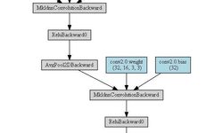
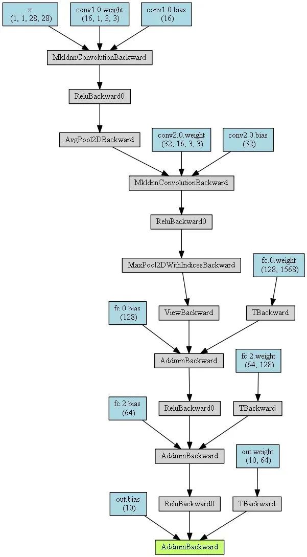
With the basic neural network established, we will visualize the above convolutional neural network using the HiddenLayer and PyTorchViz libraries.
It should be noted that both of these libraries are developed based on Graphviz, so if you haven’t installed it and added the environment variable on your computer, please install the Graphviz tool yourself, installation tutorial
1.1 Visualizing the Network with HiddenLayer
First, of course, install the library, open cmd, and enter:
pip install hiddenlayer
The basic program for drawing is as follows:
 import hiddenlayer as h
 vis_graph = h.build_graph(MyConvNet, torch.zeros([1 ,1, 28, 28]))   # Get the object for drawing the image
 vis_graph.theme = h.graph.THEMES["blue"].copy()     # Specify theme color
 vis_graph.save("./demo1.png")   # Save image path
The effect is as follows:
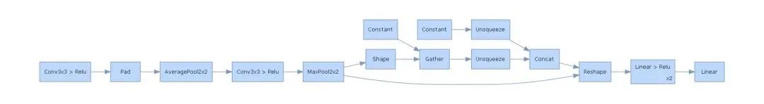
1.2 Visualizing the Network with PyTorchViz
First install the library:
pip install torchviz
Here, we only use the visualization function make_dot() to obtain the drawing object, which is similar to HiddenLayer, but different in that PyTorch allows specifying an input value and prediction value for the network before drawing.
 from torchviz import make_dot
 x = torch.randn(1, 1, 28, 28).requires_grad_(True)  # Define an input value for the network
 y = MyConvNet(x)    # Get the network's prediction value

 MyConvNetVis = make_dot(y, params=dict(list(MyConvNet.named_parameters()) + [("x", x)]))
 MyConvNetVis.format = "png"
 # Specify the folder where the file will be generated
 MyConvNetVis.directory = "data"
 # Generate file
 MyConvNetVis.view()
Open the data folder in the same root directory as the above code, there will be a .gv file and a .png file, where the .gv file is the script code generated by the Graphviz tool, and the .png is the image generated by compiling the .gv file, just open the .png file.
By default, the above program will automatically open the .png file after running
Generated image:
2. Visualization of the Training Process
Observing the changes in our network’s loss function or accuracy at each step can effectively help us assess the quality of the current training process. If we can visualize these processes, our judgment accuracy and comfort will also increase.
This section mainly discusses how to visualize the training process using the visualization tools tensorboardX and the HiddenLayer we just used.
To train the network, we first import the data needed for training, here we will import the MNIST dataset and perform some basic data processing before training.
 import torchvision
 import torch.utils.data as Data
 # Prepare the MNIST dataset for training
 train_data = torchvision.datasets.MNIST(
     root = "./data/MNIST",  # Path to extract data
     train=True, # Use the training data in MNIST
     transform=torchvision.transforms.ToTensor(),    # Convert to torch.tensor
     download=False   # If this is the first run, set to True to download the dataset to the root directory
 )

 # Define loader
 train_loader = Data.DataLoader(
     dataset=train_data,
     batch_size=128,
     shuffle=True,
     num_workers=0
 )

 test_data = torchvision.datasets.MNIST(
     root="./data/MNIST",
     train=False,    # Use test data
     download=False
 )

 # Normalize test data to 0-1
 test_data_x = test_data.data.type(torch.FloatTensor) / 255.0
 test_data_x = torch.unsqueeze(test_data_x, dim=1)
 test_data_y = test_data.targets

 # Print the shape of test data and training data
 print("test_data_x.shape:", test_data_x.shape)
 print("test_data_y.shape:", test_data_y.shape)

 for x, y in train_loader:
     print(x.shape)
     print(y.shape)
     break
Result:
 test_data_x.shape: torch.Size([10000, 1, 28, 28])
 test_data_y.shape: torch.Size([10000])
 torch.Size([128, 1, 28, 28])
 torch.Size([128])
2.1 Visualizing the Training Process with tensorboardX
tensorboard is a deep learning visualization tool developed by Google as part of the TensorFlow deep learning framework. With the efforts of the PyTorch team, they have developed tensorboardX to allow PyTorch users to also enjoy the benefits of tensorboard.
First, install the relevant libraries:
 pip install tensorboardX
 pip install tensorboard
And add the folder path where tensorboard.exe is located to the environment variable path (for example, if the path of my tensorboard.exe is D:\Python376\Scripts\tensorboard.exe, then add D:\Python376\Scripts to the path).
Below is the usage process of tensorboardX. The basic usage is to first obtain a log writer object through the SummaryWriter class under tensorboardX. Then, through a set of methods of this object, add events to the log, generating corresponding images, and finally start the front-end server to see the final result in localhost.
The code to train the network and visualize the training process is as follows:
from tensorboardX import SummaryWriter
logger = SummaryWriter(log_dir="data/log")
# Get optimizer and loss function
optimizer = torch.optim.Adam(MyConvNet.parameters(), lr=3e-4)
loss_func = nn.CrossEntropyLoss()
log_step_interval = 100 # Interval for logging steps
for epoch in range(5):
print("epoch:", epoch)
# Each round traverses the data loader once
for step, (x, y) in enumerate(train_loader):
# Forward computation -> calculate loss function -> (from loss function) backpropagation -> update network
predict = MyConvNet(x)
loss = loss_func(predict, y)
optimizer.zero_grad() # Clear gradients (optional)
loss.backward() # Backpropagation to compute gradients
optimizer.step() # Update network
global_iter_num = epoch * len(train_loader) + step + 1 # Calculate the current step from the start of training (global iteration count)
if global_iter_num % log_step_interval == 0:
# Output to console
print("global_step:{}, loss:{:.2}".format(global_iter_num, loss.item()))
# First log entry: loss function - global iteration count
logger.add_scalar("train loss", loss.item() ,global_step=global_iter_num)
# Predict on the test set and calculate accuracy
test_predict = MyConvNet(test_data_x)
_, predict_idx = torch.max(test_predict, 1) # Calculate the index of the maximum value after softmax, i.e., the prediction result
acc = accuracy_score(test_data_y, predict_idx)
# Second log entry: accuracy - global iteration count
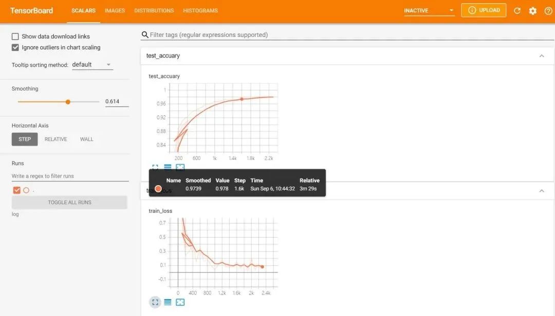
logger.add_scalar("test accuracy", acc.item(), global_step=global_iter_num)
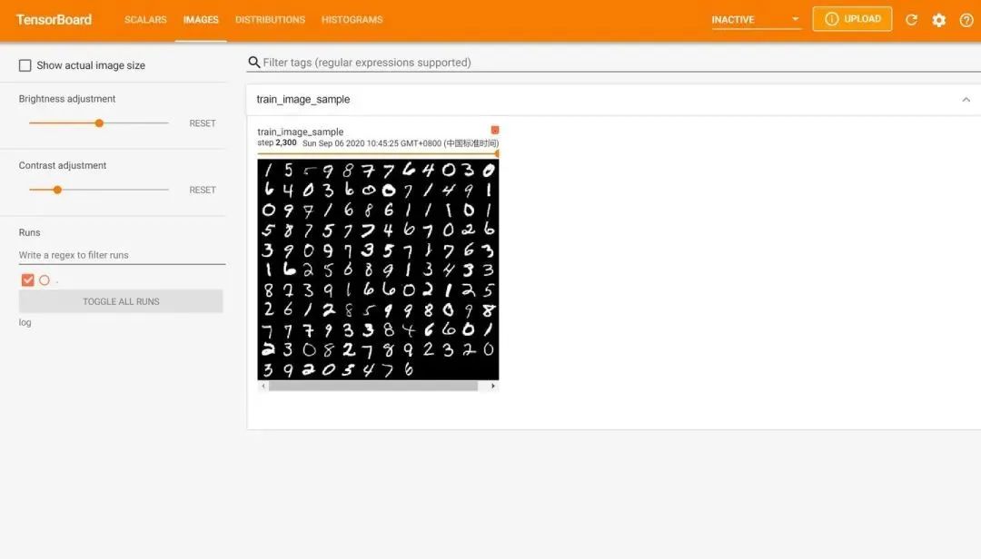
# Third log entry: 128 images in this batch
img = vutils.make_grid(x, nrow=12)
logger.add_image("train image sample", img, global_step=global_iter_num)
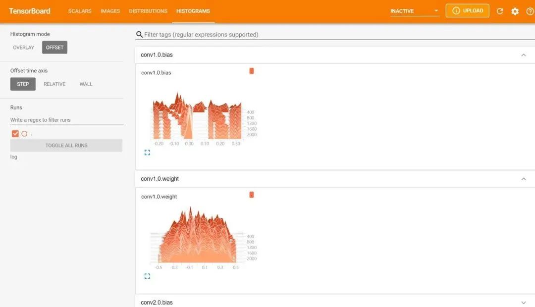
# Fourth log entry: histogram of parameter distribution in the network
for name, param in MyConvNet.named_parameters():
logger.add_histogram(name, param.data.numpy(), global_step=global_iter_num)
After running, we enter the command tensorboard --logdir="./data/log" in cmd, in the directory at the same level as the code (if you are using PyCharm, you can do this in the terminal within PyCharm) to start the server.
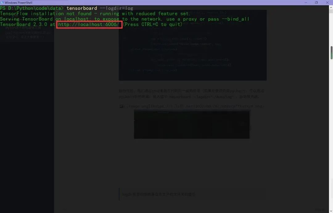
The parameter after logdir is the path to the log file folder
Then visit the URL in the red box in Google Chrome to obtain the visualization interface. Click on the page controls above to view the images generated by add_scalar, add_image, and add_histogram, and everything runs smoothly.
Here are some errors encountered by the author when installing and using tensorboard.
As a user who has never installed TensorFlow on Windows, the author will now start to step on some pits. After stepping on them, I will present several possible errors.
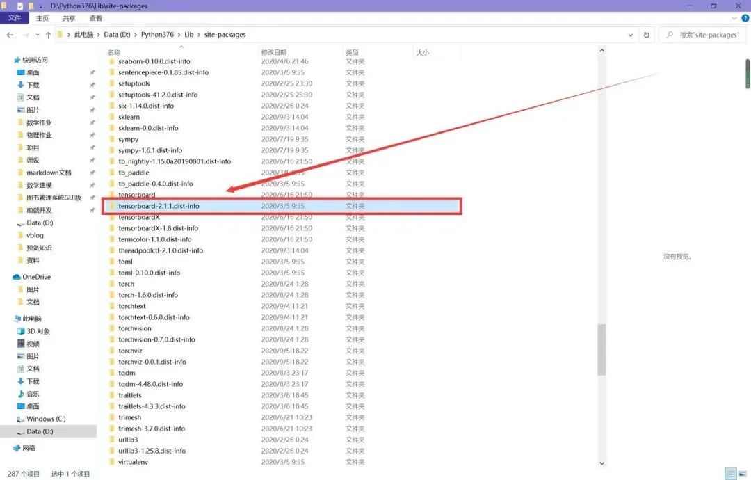
The first error, when running tensorboard --logdir="./data/log", an error occurs stating that there are duplicate tensorboard packages.
Solution: Find the site-packages (if you installed globally like me, find the site-packages in the interpreter’s root directory, if installed in the project’s virtual environment, find the site-packages in the project), and delete the folder marked in red in the image below.
The second error, after resolving the first error, running the command again still results in an error with encoding issues. Since the author has done some front-end work, I was once told that project paths cannot contain Chinese characters, otherwise there will be encoding errors. The previous error involved starting the front-end server, so I thought of addressing it from the file name.
Solution: Ensure that the file paths involved in the command and all programs do not contain Chinese characters. The author’s computer name contains Chinese characters, and the tensorboard log file is suffixed with the local computer name, so I changed the computer name to English, restarted, and then the command worked fine.
2.2 Visualizing the Training Process with HiddenLayer
The images from tensorboard are stunning, but the usage process is relatively cumbersome compared to other toolkits, so it is generally unnecessary to use tensorboard for small networks.
 import hiddenlayer as hl
 import time

 # Record metrics during training
 history = hl.History()
 # Use canvas for visualization
 canvas = hl.Canvas()

 # Get optimizer and loss function
 optimizer = torch.optim.Adam(MyConvNet.parameters(), lr=3e-4)
 loss_func = nn.CrossEntropyLoss()
 log_step_interval = 100      # Interval for logging steps

 for epoch in range(5):
     print("epoch:", epoch)
     # Each round traverses the data loader once
     for step, (x, y) in enumerate(train_loader):
         # Forward computation -> calculate loss function -> (from loss function) backpropagation -> update network
         predict = MyConvNet(x)
         loss = loss_func(predict, y)
         optimizer.zero_grad()   # Clear gradients (optional)
         loss.backward()     # Backpropagation to compute gradients
         optimizer.step()    # Update network
         global_iter_num = epoch * len(train_loader) + step + 1  # Calculate the current step from the start of training (global iteration count)
         if global_iter_num % log_step_interval == 0:
             # Output to console
             print("global_step:{}, loss:{:.2}".format(global_iter_num, loss.item()))
             # On the test set, predict and calculate accuracy
             test_predict = MyConvNet(test_data_x)
             _, predict_idx = torch.max(test_predict, 1)  # Calculate the index of the maximum value after softmax, i.e., the prediction result
             acc = accuracy_score(test_data_y, predict_idx)

             # Create a log dictionary indexed by epoch and step
             history.log((epoch, step),
                         train_loss=loss,
                         test_acc=acc,
                         hidden_weight=MyConvNet.fc[2].weight)

             # Visualization
             with canvas:
                 canvas.draw_plot(history["train_loss"])
                 canvas.draw_plot(history["test_acc"])
                 canvas.draw_image(history["hidden_weight"])
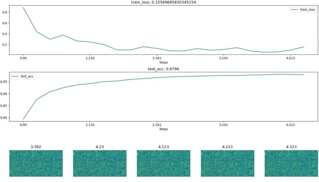
Unlike tensorboard, hiddenlayer dynamically generates images during the program’s execution, rather than after the model training is complete
Below is a screenshot of the model training at a certain moment:
3. Using Visdom for Visualization
Visdom is a visualization tool developed by Facebook for PyTorch. Similar to tensorboard, visdom also implements visualization by starting a front-end server locally, but in specific operations, visdom is more similar to matplotlib.pyplot, making it very flexible to use.
First, install the visdom library and fill in the gaps. Since starting the front-end server requires a lot of dependencies, it may be slow the first time you start it (dependencies for the front-end framework need to be downloaded), please see here for solutions.
First, import the required third-party libraries:
 from visdom import Visdom
 from sklearn.datasets import  load_iris
 import torch
 import numpy as np
 from PIL import Image
In matplotlib, users can draw using the plt object, and in visdom, a drawing object is also needed. We obtain it by vis = Visdom(). When drawing, since we will plot several images at once, visdom requires users to specify the current drawing window name (the win parameter); in addition, to display the images in blocks, users also need to specify the drawing environment env, which means that images with the same parameter will be displayed on the same page.
Draw line graphs (equivalent to plt.plot in matplotlib):
 # Data needed for drawing
 iris_x, iris_y = load_iris(return_X_y=True)

 # Get drawing object, equivalent to plt
 vis = Visdom()

 # Add line graph
 x = torch.linspace(-6, 6, 100).view([-1, 1])
 sigmoid = torch.nn.Sigmoid()
 sigmoid_y = sigmoid(x)
 tanh = torch.nn.Tanh()
 tanh_y = tanh(x)
 relu = torch.nn.ReLU()
 relu_y = relu(x)
 # Connect three tensors
 plot_x = torch.cat([x, x, x], dim=1)
 plot_y = torch.cat([sigmoid_y, tanh_y, relu_y], dim=1)
 # Draw line graph
 vis.line(X=plot_x, Y=plot_y, win="line plot", env="main",
          opts={
              "dash" : np.array(["solid", "dash", "dashdot"]),
              "legend" : ["Sigmoid", "Tanh", "ReLU"]
          })
Draw scatter plots:
 # Draw 2D and 3D scatter plots
 # Parameter Y specifies the distribution of points, win specifies the window name of the image, env specifies the environment of the image, opts specifies some styles through a dictionary
 vis.scatter(iris_x[ : , 0 : 2], Y=iris_y+1, win="windows1", env="main")
 vis.scatter(iris_x[ : , 0 : 3], Y=iris_y+1, win="3D scatter", env="main",
             opts={
                 "markersize" : 4,   # Size of points
                 "xlabel" : "Feature 1",
                 "ylabel" : "Feature 2"
             })
Draw stem-and-leaf plots:
 # Add stem-and-leaf plot
 x = torch.linspace(-6, 6, 100).view([-1, 1])
 y1 = torch.sin(x)
 y2 = torch.cos(x)

 # Connect tensors
 plot_x = torch.cat([x, x], dim=1)
 plot_y = torch.cat([y1, y2], dim=1)
 # Draw stem-and-leaf plot
 vis.stem(X=plot_x, Y=plot_y, win="stem plot", env="main",
          opts={
              "legend" : ["sin", "cos"],
              "title" : "Stem-and-leaf plot"
          })
Draw heat maps:
 # Calculate the correlation matrix of feature vectors in the iris dataset
 iris_corr = torch.from_numpy(np.corrcoef(iris_x, rowvar=False))
 # Draw heatmap
 vis.heatmap(iris_corr, win="heatmap", env="main",
             opts={
                 "rownames" : ["x1", "x2", "x3", "x4"],
                 "columnnames" : ["x1", "x2", "x3", "x4"],
                 "title" : "Heatmap"
             })
Visualize images, here we use a custom env name MyPlotEnv:
 # Visualize images
 img_Image = Image.open("./example.jpg")
 img_array = np.array(img_Image.convert("L"), dtype=np.float32)
 img_tensor = torch.from_numpy(img_array)
 print(img_tensor.shape)

 # This time env is custom
 vis.image(img_tensor, win="one image", env="MyPlotEnv",
           opts={
               "title" : "An Image"
           })
Visualize text, also drawn in MyPlotEnv:
 # Visualize text
 text = "hello world"
 vis.text(text=text, win="text plot", env="MyPlotEnv",
          opts={
              "title" : "Visualized Text"
          })
Run the above code and then start the server by entering python3 -m visdom.server in the terminal. Then access the URL returned in the terminal in Google Chrome to see the images.
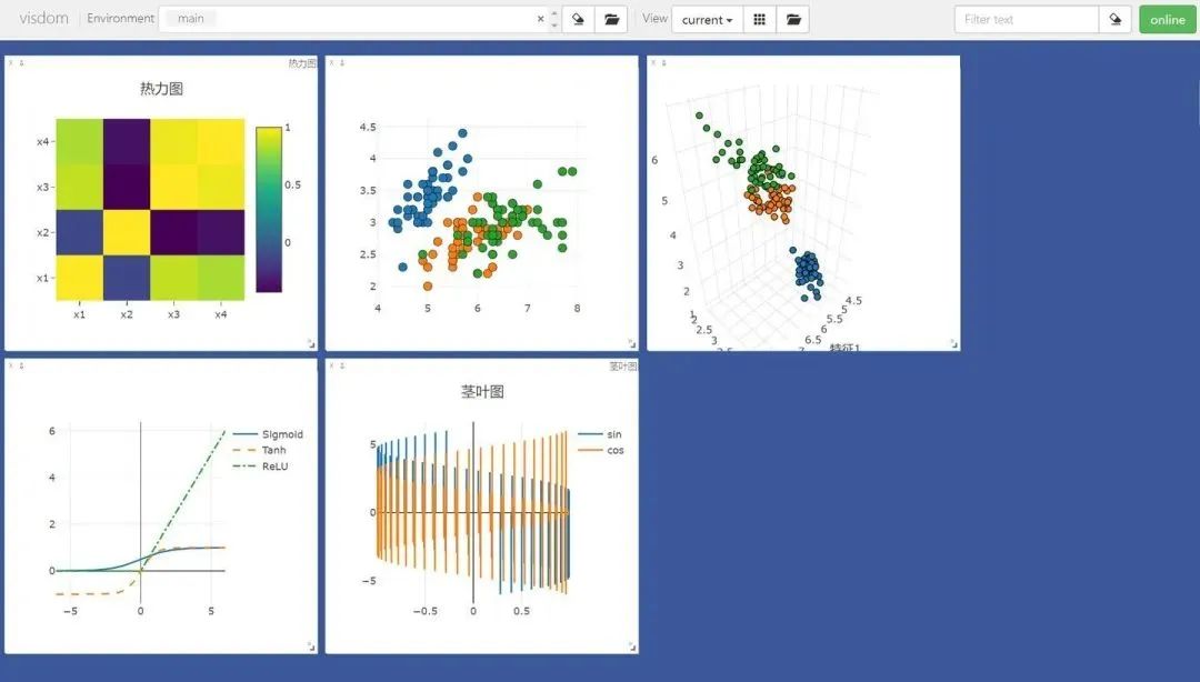
By entering different env parameters in the Environment, you can see the images we drew in different environments. This is particularly useful for classification galleries.
Press Ctrl+C in the terminal to terminate the front-end server.
Further
It is important to note that if your front-end server is stopped, all images will be lost because the data for these images resides in memory and has not been dumped to local disk. So how can we save the current visualization results in visdom and reuse them in the future? It’s quite simple. For example, I now have a bunch of hard-earned Mel spectrograms:

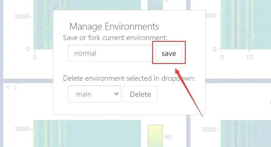
Click Manage Views

Click fork -> save: (here I only save the env named normal)
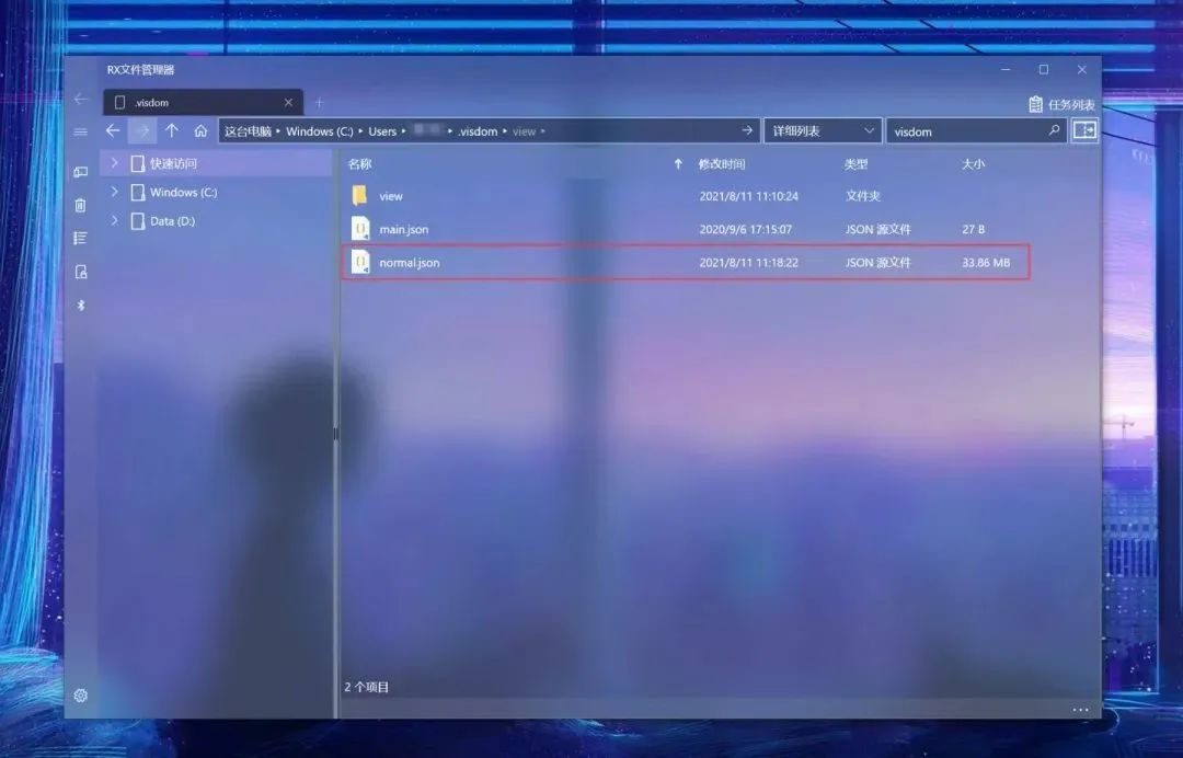
Then, in your User directory (Windows is C:\Users\account\.visdom folder, Linux is in ~/.visdom folder), you can see the saved env:
It is saved in JSON file format, so if you shut down the current front-end server after saving your precious data, the image data will not be lost.
Now, after saving your valuable data, please close your visdom front-end server. Then restart it.
How to view the saved data? Very simple, the next time you open the visdom front-end, visdom will read all the saved data from the .visdom folder during initialization, meaning you can directly start visdom and see the previously saved data without doing anything else!
So how to reuse the saved data? Since you know where the saved data is located, you can directly read this data file using Python’s JSON package and parse it. This is method one, demonstrated as follows:
import json

with open(r"...\.visdom\normal.json", "r", encoding="utf-8") as f:
    dataset : dict = json.load(f)

jsons : dict = dataset["jsons"]      # This stores the data you want to recover
reload : dict = dataset["reload"]    # This stores data about window sizes

print(jsons.keys())     # View all wins
out:
dict_keys(['jsons', 'reload'])
dict_keys(['1.wav', '2.wav', '3.wav', '4.wav', '5.wav', '6.wav', '7.wav', '8.wav', '9.wav', '10.wav', '11.wav', '12.wav', '13.wav', '14.wav'])
However, this approach is not very elegant, so visdom has encapsulated a second method. You can certainly check the available envs by accessing the .visdom folder, but you can also do this:
from visdom import Visdom

vis = Visdom()
print(vis.get_env_list())
out:
Setting up a new session...
['main', 'normal']
After obtaining the available environment names, you can use the get_window_data method to get the image data under a specified env and win. Note that this method returns str, so it needs to be parsed with JSON:
from visdom import Visdom
import json

vis = Visdom()

window = vis.get_window_data(win="1.wav", env="normal")
window = json.loads(window)         # window is str, needs to be parsed into a dictionary

content = window["content"]
data = content["data"][0]
print(data.keys())
out:
Setting up a new session...
dict_keys(['z', 'x', 'y', 'zmin', 'zmax', 'type', 'colorscale'])
By indexing these keys, it should not be difficult to reuse the original image data.
Download 1: OpenCV-Contrib Extension Module Chinese Version Tutorial

Reply to "Chinese Tutorial for Extension Modules" in the background of the "Beginner Learning Vision" public account to download the first Chinese version of the OpenCV extension module tutorial, covering installation of extension modules, SFM algorithms, stereo vision, target tracking, biological vision, super-resolution processing, and more than twenty chapters of content.

Download 2: Python Vision Practical Project 52 Lectures

Reply to "Python Vision Practical Project" in the background of the "Beginner Learning Vision" public account to download 31 practical vision projects including image segmentation, mask detection, lane line detection, vehicle counting, eyeliner addition, license plate recognition, character recognition, emotion detection, text content extraction, face recognition, etc., to help quickly learn computer vision.

Download 3: OpenCV Practical Project 20 Lectures

Reply to "OpenCV Practical Project 20 Lectures" in the background of the "Beginner Learning Vision" public account to download 20 practical projects based on OpenCV, achieving advanced learning of OpenCV.

Discussion Group

Welcome to join the reader group of the public account to communicate with peers. Currently, there are WeChat groups for SLAM, 3D vision, sensors, autonomous driving, computational photography, detection, segmentation, recognition, medical imaging, GAN, algorithm competitions, etc. (these will gradually be subdivided). Please scan the WeChat number below to join the group, and note: "Nickname + School/Company + Research Direction", for example: "Zhang San + Shanghai Jiao Tong University + Vision SLAM". Please follow the format, otherwise, you will not be approved. After successfully adding, you will be invited to the relevant WeChat group according to your research direction. Please do not send advertisements in the group, otherwise, you will be removed from the group. Thank you for your understanding~