Choosing the Right Loss Function in PyTorch: MAE, MSE, Huber

Direct Results:

Image excerpted from the end of this article

Main Text:

In both machine learning and deep learning fields, the loss function is a very important concept. There are many different types of loss functions, and different loss functions need to be selected based on specific models and application scenarios. Choosing the model’s loss function is one of the most fundamental and critical skills for algorithm engineers in practical applications. Recently, while learning PyTorch, I referred to many documentation and excellent posts, summarizing how to choose the appropriate loss function for application scenarios, compare the advantages and disadvantages of different loss functions, and related PyTorch code, for my learning record and to facilitate my review. The content includes:

1. Basic Knowledge (Loss Function, Training Objectives, Training Methods, PyTorch)
2. Regression Model Loss Functions (Advantages and Disadvantages of MSE, MAE, Huber Loss Functions, Summary of Application Scenarios)
3. Classification Model Loss Functions (Entropy, Maximum Likelihood)

1. Basic Knowledge

Before understanding the principles of choosing various loss functions, let’s review some basic concepts related to loss functions, model training, and training methods.

Loss Function: Used to measure the degree of deviation between the model’s predicted value f(x) and true value y. The basic and advanced requirements for choosing a loss function are as follows:

• Basic Requirement: Used to measure the closeness between the model output distribution and the sample label distribution.
• Advanced Requirement: Accurately describes the closeness between the model output distribution and the sample labels under uneven sample distribution conditions.

Model Training: The training process is essentially the optimization (minimization) of the loss function, making f(x) as close as possible to y. In fact, it is the process of fitting model parameters (for example, using least squares or gradient descent to solve parameters in regression models), and can also be understood as the process of solving the model (for example, using the maximum likelihood method to solve parameters in probabilistic models). This is fundamentally not much different from the process of solving parameters in other mathematical modeling.

Common Training Methods: Gradient descent algorithm to find the minimum of a function.

Generally, loss functions directly calculate the data of a batch, so the returned loss results are vectors with dimensions of batch_size. It is worth noting that many loss functions in PyTorch have two boolean parameters: size_average and reduce, specifically:

• If reduce = False, then the size_average parameter is invalid, and it directly returns the loss in vector form;

• If reduce = True, then the loss returns a scalar.

• If size_average = True, returns loss.mean();
• If size_average = True, returns loss.sum();

To better understand the definition of loss functions, the following code sets both parameters to False:

Generally speaking, commonly used loss functions in engineering practice can be roughly divided into two major application scenarios: Regression and Classification.

2. Regression Models

1. nn.MSELoss (Mean Square Error)

The mean square loss function has the following mathematical form:

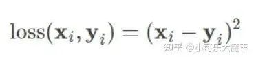
Here, the dimensions of loss, x, and y are the same, which can be vectors or matrices, with i as the index.

Using y-f(x) as the x-axis and MSE as the y-axis, we can plot the graph of the loss function:

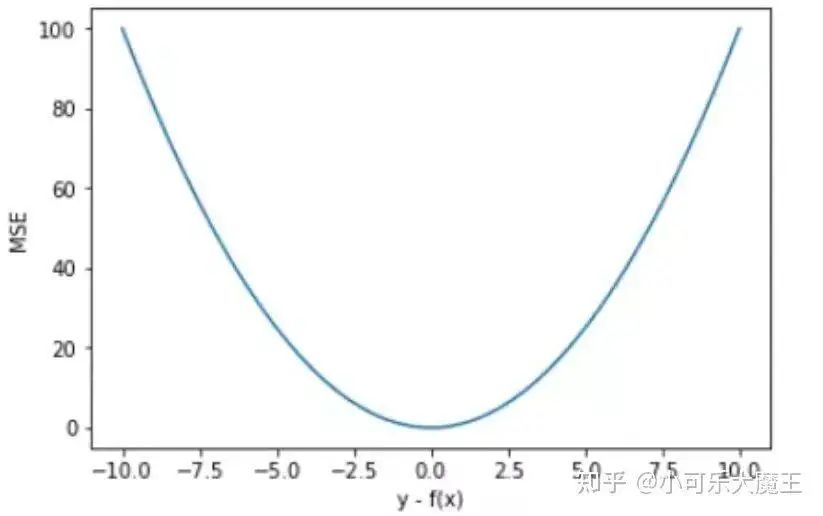
The characteristics of the MSE curve are smooth, continuous, and differentiable, making it easy to use with the gradient descent algorithm. The square error has a property that when the difference between yi and f(xi) is greater than 1, it increases the error; when the difference is less than 1, it decreases the error. This is determined by the nature of squaring. In other words, MSE punishes larger errors (>1) more and smaller errors (<1) less. For example, if the true value is 1 and there is one prediction of 1000 among ten predictions, while the others are around 1, the loss value is primarily determined by 1000.

Advantages: Quick Convergence – As the error decreases, the gradient of MSE also decreases, which is beneficial for the function’s convergence; even with a fixed learning rate, the function can converge to the minimum value quickly.

Disadvantages: Highly Sensitive to Outliers – From the perspective of training, the model tends to penalize larger points more, giving them greater weight and ignoring the role of smaller points, which cannot avoid the gradient explosion problem that outliers may cause. If there are outliers in the sample, MSE assigns higher weights to outliers, but at the cost of sacrificing the predictive performance of other normal data points, which leads to decreased overall model performance.

PyTorch code implementation:

import torch
from torch.autograd import Variable
import torch.nn as nn
import torch.nn.functional as F

# Choose loss function MSE
loss_func=torch.nn.MSELoss()
# Randomly generate data
input=torch.autograd.Variable(torch.randn(3,4))
targets=torch.autograd.Variable(torch.randn(3,4))

# Calculate loss
loss = loss_func(input, target)
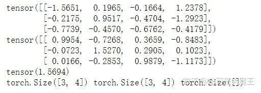
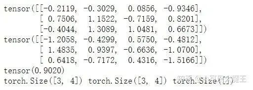
print(input); print(target); print(loss)
print(input.size(), target.size(), loss.size())

Output:

2. nn.L1Loss & MAE (Mean Absolute Error)

Absolute error and L1 error, both refer to the average distance between the model’s predicted value f(x) and the sample’s true value y, with the following formula:

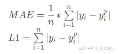
It requires that the dimensions of x and y be the same (which can be vectors or matrices), and the resulting loss dimension is also correspondingly the same. Here, the index i represents the i-th element.

Using y-f(x) as the x-axis and MAE as the y-axis, we can plot the graph of the loss function:

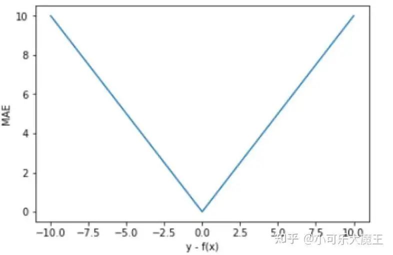
The MAE curve is V-shaped, continuous but not differentiable at y-f(x)=0, making it difficult for computers to differentiate. Moreover, in most cases, the gradient is equal, which means that even for small loss values, the gradient is still large, hindering the convergence of the function and the learning of the model.

Advantages: Since MAE calculates absolute errors, regardless of whether y-f(x)>1 or y-f(x)<1, without the effect of the square term, the punishment is the same. Thus, compared to MSE, MAE is less sensitive to outliers and can better represent the distribution of normal data, showing better robustness.

Disadvantages: During training, the gradient of MAE is always large and is continuous but not differentiable at the point zero, meaning that even for small loss values, the gradient is still large. This hinders the convergence of the function and the learning of the model, leading to a slow learning speed and may also cause the model to miss the global minimum when using gradient descent for training.

The MAE curve is continuous but not differentiable at (y-f(x)=0).

The code implementation is determined by the parameter reduction of torch.nn.L1Loss. When the parameter reduction:

• Choosing ‘mean’ or ‘none’ is MAE;
• Choosing ‘sum’ is L1 loss;

loss_func = torch.nn.L1Loss()
input = torch.autograd.Variable(torch.randn(3,4))
target = torch.autograd.Variable(torch.randn(3,4))
loss = loss_func(input, target)
print(input); print(target); print(loss)
print(input.size(), target.size(), loss.size())

Output:

3. nn.SmoothL1Loss (Huber Loss Function)

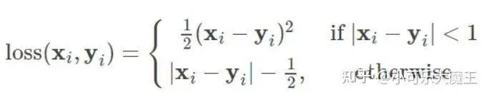
Huber loss function (smooth average absolute error) combines both square error loss.

The Huber function is a combination of MAE and MSE, and it is also differentiable when its function value is 0. It includes a hyperparameter δ, where the value of δ determines whether Huber emphasizes MSE or MAE’s superior performance.

• When δ ~ 0, the Huber loss approaches MSE;
• When δ ~ ∞ (a very large number), the Huber loss approaches MAE.

Taking δ = 0.1 and δ = 10, we can plot the corresponding graphs of the Huber Loss loss function:

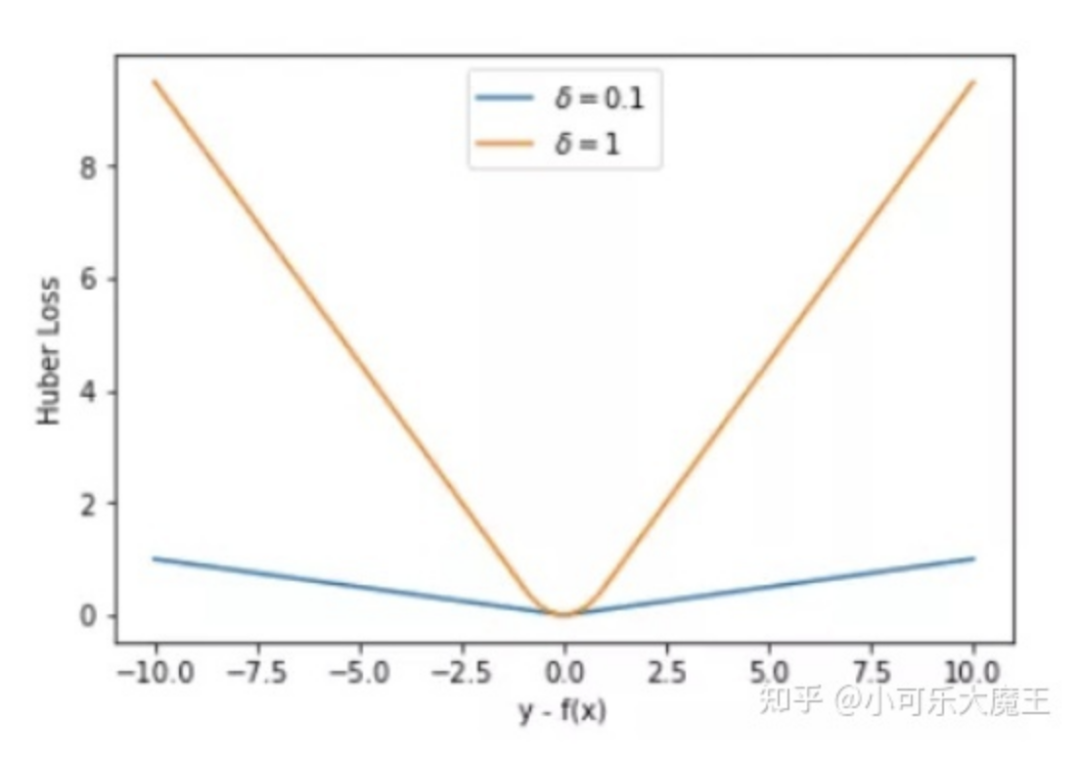
    When |y−f(x)| > δ, the gradient is approximately δ, ensuring that the model updates its parameters at a faster rate.
    When |y−f(x)| ≤ δ, the gradient gradually decreases, allowing the model to more accurately obtain the global optimal value.

This function is essentially a piecewise function, smooth in the interval [-1,1], thus solving the non-smooth problem of MAE, and in the intervals [-∞,1) and (1,+∞], it addresses the gradient explosion problem that MSE may cause due to outliers. Specifically:

The Huber function reduces the gradient around its minimum value, and compared to MSE, it is more robust to outliers. The Huber function possesses the advantages of both MSE and MAE, mitigating the excessive sensitivity to outliers while achieving differentiability everywhere.

Advantages: It possesses the advantages of both MSE and MAE, mitigating excessive sensitivity to outliers while achieving differentiability everywhere, and converges faster than MAE.

• Compared to the MAE loss function, it can converge faster;
• Compared to the MSE loss function, it is less sensitive to outliers and anomalies, with relatively smaller gradient changes, making it less likely to produce strange results during training.

Note: The hyperparameter δ needs to be selected during training, often using cross-validation to select an appropriate hyperparameter δ, as the selection of hyperparameters directly affects the quality of training results.

Cross-validation: https://blog.csdn.net/weixin_40475450/article/details/80578943

Code implementation:

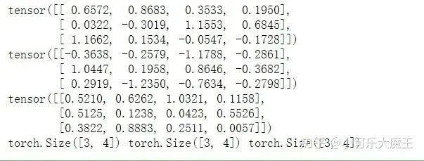
loss_func = torch.nn.SmoothL1Loss(reduce=False, size_average=False)
input = torch.autograd.Variable(torch.randn(3,4))
target = torch.autograd.Variable(torch.randn(3,4))
loss = loss_func(input, target)
print(input); print(target); print(loss)
print(input.size(), target.size(), loss.size())

Code results:

Summary: How to Choose the Appropriate Loss Function in Industrial Applications

• From the perspective of error: MSE can be used to evaluate the degree of data variation, while MAE better reflects the actual situation of prediction value errors.
• From the perspective of outliers: If outliers are merely damaged during data extraction or errors in sampling during cleaning, they need not be overly concerned, and we should choose MAE. However, if outliers are actual data or important anomalies that need to be detected, we should choose MSE.
• From the perspective of convergence speed: MSE > Huber > MAE.
• From the perspective of solving gradient complexity: MSE is superior to MAE, and the gradient is also dynamically changing, allowing MSE to accurately reach convergence quickly.
• From the model perspective: For most CNN networks, we generally use MSE rather than MAE, as training CNN networks places great importance on training speed. For border prediction regression problems, we can usually choose square loss functions, but the drawback of square loss functions is that when there are outliers, these points will constitute the main part of the loss. For object detection, Fast R-CNN adopts a slightly moderated absolute loss function (smooth L1 loss), which increases linearly with error rather than quadratically.