Click the “AI Park” above to follow the public account, and choose to add a “star” or “top”
Author: Suvro Banerjee
Translated by: ronghuaiyang
In NLP today, word vectors are indispensable. Word vectors provide us with a very good vector representation of words, allowing us to represent all words with a fixed-length vector, and also represent the contextual relationships between words. Isn’t that amazing? So, how did such a magical thing come about? This article will clarify everything step by step. Although there are some formulas, it is still very easy to understand overall, so let’s take a look.
Let’s Unveil Word2Vec Through Reasoning, Examples, and Mathematics
Introduction
The Word2Vec model is used to learn the vector representation of words, known as “word embeddings.” This is usually done as a preprocessing step, after which the learned vectors are input into a discriminative model (usually an RNN) to generate predictions and accomplish various interesting tasks.
Why Learn Word Embeddings
Image and audio processing systems use rich high-dimensional datasets, where image data is encoded as vectors composed of the intensity of individual pixels, thus all information is encoded in the data, allowing for the establishment of relationships between various entities in the system (cats and dogs).
However, in natural language processing systems, traditionally it treats words as discrete atomic symbols, so “cat” can be represented as Id537, and “dog” as Id143. These encodings are arbitrary and do not provide the system with useful information about the relationships that may exist between various symbols. This means that the model has very little knowledge about “cats” when processing data about “dogs” (like they are both animals, have four legs, are pets, etc.).
Representing words as unique, discrete IDs also leads to data sparsity, which often means we may need more data to successfully train statistical models. Using vector representations can overcome some of these obstacles.
For example:
Traditional natural language processing methods involve a lot of domain knowledge about linguistics itself. Understanding terms like phonemes and morphemes is quite standard, as there are entire language courses dedicated to their study. Let’s see how traditional NLP understands the following word.
Suppose our goal is to gather some information about this word (describe its sentiment, find its definition, etc.). Utilizing our linguistic domain knowledge, we can break this word down into three parts.
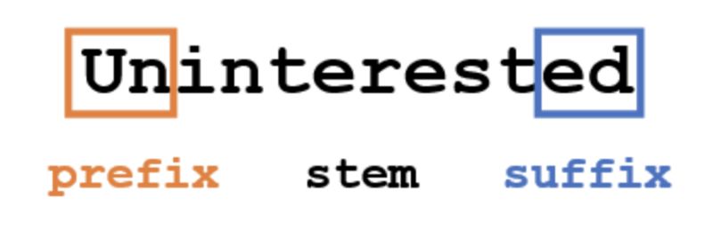
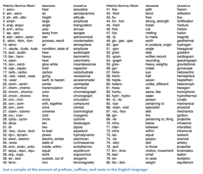
We know the prefix “un” means opposite or contrary, and “ed” can specify the time period of the word (past tense). By recognizing the meaning of the stem “interest,” we can easily deduce the definition and sentiment of the entire word. Seems simple, right? However, when you consider all the different prefixes and suffixes in English, it requires a very skilled linguist to understand all possible combinations and meanings.
Deep learning, at its most fundamental level, is about representation learning. Here, we will take the same approach by creating representations of words through large datasets.
Word Vectors
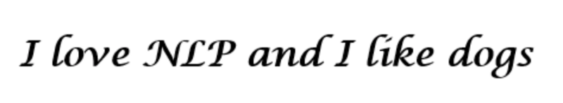
We represent each word as a d-dimensional vector. Let’s use d = 6. From this sentence, we want to create a word vector for each word.
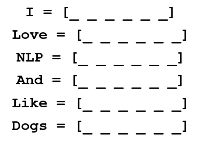
Now let’s consider how to fill these values. We want to fill in the values in such a way that the vector represents the word and its context, meaning, or semantics in some manner. One way is to create a co-occurrence matrix.
A co-occurrence matrix is a matrix that contains the counts of each word appearing next to every other word in the corpus (or training set). Let’s visualize this matrix.
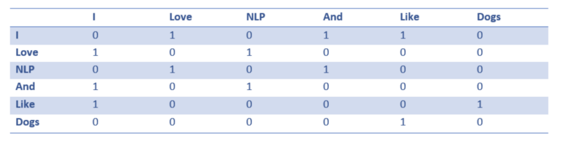
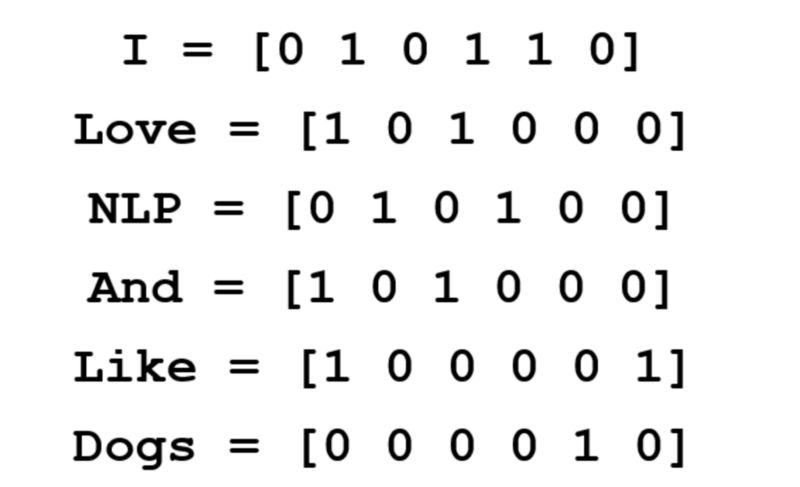
Note that through this simple matrix, we can gain very useful insights. For example, note that the words “love” and “like” both contain 1, indicating their counts with the noun (NLP and dogs), and their counts of “I” is also 1, meaning the word must be some kind of verb. With a larger dataset than a single sentence, you can imagine this similarity will become clearer, as “like,” “love,” and other synonyms will begin to have similar word vectors because they are used in similar contexts.
Now, while this is a good starting point, we notice that the dimensions of each word will grow linearly with the size of the corpus. If we have a million words (which is not very many by NLP standards), we will have a million x million sized matrix, which is very sparse (lots of 0s). This is definitely not the best in terms of storage efficiency. Significant progress has been made in finding optimal ways to represent these word vectors. One of the most famous methods is Word2Vec.
Past Methods
Vector Space Models (VSMs) represent (embed) words in a continuous vector space, where semantically similar words map to points that are close to each other (“embedded near each other”). VSMs have a long and rich history in NLP, but all methods rely, more or less, on the distributional hypothesis, which states that words that appear in the same context have similar meanings. Different methods that leverage this principle can be divided into two categories:
-
Count-based methods (like Latent Semantic Analysis)
-
Predictive methods (like Neural Probabilistic Language Models)
The distinction is:
Count-based methods compute the frequency with which a word co-occurs with neighboring words in a large text corpus, and then map these count statistics to small, dense vectors for each word.
Predictive models directly try to predict neighboring words by learning small, dense embedding vectors (considering the model’s parameters).
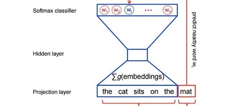
Word2Vec is an efficient predictive model that learns embeddings for words from raw text. It comes in two flavors, the Continuous Bag of Words model (CBOW) and the Skip-Gram model. Algorithmically, these models are similar; CBOW predicts the target word from the source context words, while Skip-Gram does the opposite, predicting the source context words from the target word.
In the following discussion, we will focus on the Skip-Gram model.
The Mathematics Behind It
The neural probabilistic language model uses the principle of maximum likelihood for traditional training, given the previous word h (representing “history”), using the softmax function to represent the probability of the next word wt (representing “target”), maximizing the entire probability.
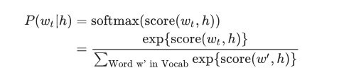
Where score(wt, h) calculates the compatibility of the target word wt with the context h (usually using the dot product).
We train this model by maximizing its log likelihood in the training set:
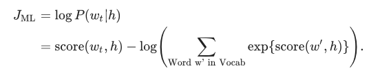
This provides a properly normalized probabilistic model for language modeling.
The same parameters can also be expressed with a slightly different formula that clearly shows the selection variable (or parameter) that is changed to maximize this objective.
Our goal is to find useful word representations for predicting the current word’s surrounding words. Specifically, we want to maximize the average log probability across the entire corpus:
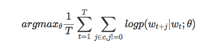
This equation essentially states that, for the current word wt, within a window of size c, observe the probability of a specific word p. This probability depends on the current word wt and a certain parameter theta (determined by our model). We want to set these parameters theta to maximize this probability across the entire corpus.
Basic Parameterization: Softmax Model
The basic Skip-Gram model defines the probability p through the softmax function, as we saw earlier. If we consider wi as a one-hot encoded vector with dimension N, and theta as an embedding matrix of dimension N * K, with N words in our vocabulary and the dimension of the learned embedding representation being K, then we can define:
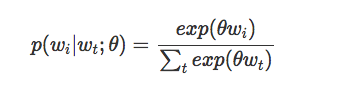
Notably, after learning, the matrix theta can be considered an embedding lookup table matrix.
Structurally, it is a simple three-layer neural network.
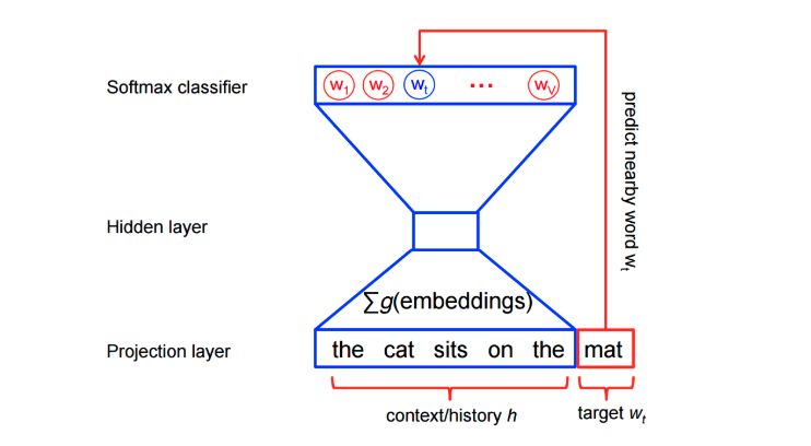
-
For example, with a 3-layer neural network (1 input layer + 1 hidden layer + 1 output layer).
-
Feed it a word to train it to predict its adjacent words.
-
Remove the last layer (output layer), keeping the input and hidden layers.
-
Now, input a word from the vocabulary. The output given at the hidden layer is the “word embedding” of the input word.
This parameterization has a major drawback, limiting its usefulness in very large companies. Specifically, we note that to compute a single forward pass of the model, we must sum over the entire vocabulary of the corpus to compute the softmax function. This is very expensive on large datasets, so we seek alternative approximations to the model for computational efficiency.
Improving Computational Efficiency
For feature learning in Word2Vec, we do not need a complete probabilistic model. The CBOW and Skip-Gram models use a binary classification objective (logistic regression) to distinguish the real target word (wt) from k fictitious (noise) words ~w in the same context.

Mathematically, the objective (for each sample) is to maximize
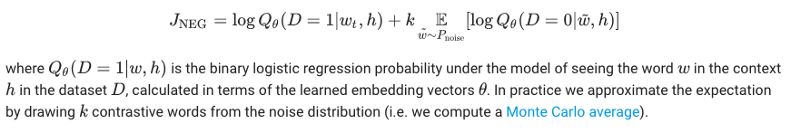
The objective is maximized when the model assigns high probabilities to real words and low probabilities to noise words. Technically, this is known as negative sampling, and the proposed updates asymptotically approximate the updates of the softmax function. But computationally, it is particularly attractive because the computation of the loss function is now scaled only by the number of noise words (k) we choose, rather than scaled by all words in the vocabulary (V), which makes training much faster. Packages like TensorFlow use a very similar loss function called Noise Contrastive Estimation (NCE) loss.
Intuition Behind the Skip-Gram Model
As an example, consider a dataset like this:
the quick brown fox jumped over the lazy dogWe first form a dataset of words and their contexts. Now, let’s continue using the ordinary definition and define “context” as the window of words to the left and right of the target word. Using a window size of 1, we obtain the dataset of (context, target) pairs.
([the, brown], quick), ([quick, fox], brown), ([brown, jumped], fox), ...Recall that Skip-Gram reverses the context and target, trying to predict each context word from the target word, so the task becomes predicting “the” and “brown” from “quick,” predicting “quick” and “fox” from “brown,” and so on.
Thus, our dataset transforms the (input, output) pairs into:
(quick, the), (quick, brown), (brown, quick), (brown, fox), ...The objective function is defined over the entire dataset, but we typically use stochastic gradient descent (SGD) to optimize it one sample (or a batch_size of samples, where usually 16 <= batch_size <= 512) at a time. Let’s look at one step of this process.
Let’s imagine in the training step, we observe the first training case above, aiming to predict the from quick. We select num_noise noise (contrast) samples from some noise distribution, typically a unigram distribution (unigram assumes each word’s occurrence is independent of all other words’ occurrences. For example, we can think of the generation process as a sequence of dice rolls), P(w)
For simplicity, let’s assume num_noise=1 and choose sheep as a noise example. Next, we compute the loss for this observed sample pair and the noise sample, so the objective at time step ‘t’ becomes:

Our goal is to update the embedding parameters theta to maximize this objective function. We achieve this by deriving the gradient of the loss concerning the embedding parameters.

Then, we take a small step in the direction of the gradient to update the embeddings. As this process is repeated across the entire training set, it effectively results in “moving” the embedding vectors of each word until the model successfully identifies real words from noise words.
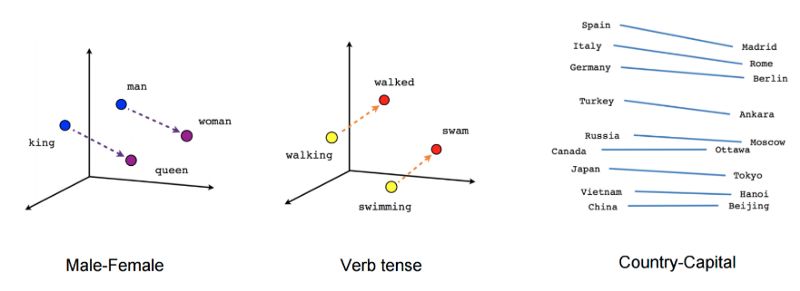
We can project the learned vectors into a two-dimensional space for visualization. When we observe these visualizations, it becomes clear that these vectors capture some general, actually very useful semantic information about words and their relationships.

Previous Highlights
1. Deep Learning Object Detection Paper Reading Roadmap and Official Implementation
2. Step-by-Step Animated Explanation of LSTM and GRU, No Math, You Will Understand!
3. To Do a Good Job, One Must First Sharpen One’s Tools, Which is the Best Python IDE for Data Science?
4. Animated Explanation of RNN; LSTM and GRU, Nothing More Intuitive Than This!
5. Heavyweight Resource! The Gospel of PyTorch, Free Deep Learning Course Using PyTorch 1.0 for Teaching, from Idiap and École Polytechnique Fédérale de Lausanne
This article can be freely reproduced, please indicate the author and original link when reprinting..

Please long press or scan the QR code to follow this public account