Understanding XGBoost Model Parameters

When companies interview candidates, the interviewers usually include HR, team leaders, and department managers. The process can be divided into two forms.

The first form is where the three interviewers interview the candidates separately. The questions may be the same or different, and each interviewer will give a conclusion based on the candidate’s performance. Finally, a comprehensive decision is made based on the conclusions from all three interviewers. This is known as Bagging.

Bagging is an abbreviation for Bootstrap AGGragatING, which is a well-known representative of parallel ensemble learning. It is based on bootstrap sampling to obtain multiple sampling sets, each of which independently trains a base learner. The final result is obtained by voting or averaging the predictions of all base learners. A typical representative of Bagging is Random Forests.

The second form is a group interview. HR, team leaders, and department managers participate in the interview simultaneously. HR first asks a few questions, the team leader asks additional questions based on the candidate’s responses to HR, and finally, the department manager asks further questions based on the team leader’s questions. The final decision on whether to accept the candidate is made based on the scores given by the three interviewers. This is known as Boosting.

Boosting is a serial ensemble learning algorithm that can elevate weak learners to strong learners. According to [Zhou Zhihua, Machine Learning]: First, a base learner is trained from the initial training set, and then the training sample distribution is adjusted based on the performance of the base learner. This means that training samples that were incorrectly classified by the previous base learner receive more attention in subsequent iterations. Then, the next base learner is trained based on the adjusted sample distribution. This process is repeated until the number of base learners reaches a predetermined value, and finally, these base learners are combined in a weighted manner. Typical representatives of Boosting include AdaBoost and GBDT series (XGBoost, LightGBM, CatBoost). GBDT stands for Gradient Boosting Decision Tree, and it is also known as MART (Multiple Additive Regression Tree). If it is a regression task, it is referred to as the Gradient Boosting Regression Tree. Different Boosting algorithms adjust the distribution in different ways. For example, the AdaBoost algorithm updates the sample weights in each iteration, increasing the weights of misclassified samples, while in GBDT, it updates the regression target by using the negative gradient of the loss function of the new iteration model as the label to train a new weak classifier, ultimately achieving model updates.. When the loss function is the squared loss function, the negative gradient of the current model’s loss function is exactly equal to the residual. At this time, each new base learner established in each round reduces the residual.Gradient is a mathematical concept (a vector whose directional derivative is maximized in that direction, and its magnitude is exactly the maximum directional derivative). The gradient direction of a function is the direction in which the function increases the fastest, while the negative gradient direction is the direction in which the function decreases the fastest.

Unlike the parallel Bagging, Boosting trains base learners one after another (serially), where each base learner makes decisions based on correcting the biases of the previous learners. The parameter settings of the later model depend on the predictions of the previous model. Bagging uses a replayable Bootstrap sampling method to select each training set from the original dataset, and the training sets are relatively independent of each other. In contrast, in Boosting, the training set for each round does not change; only the weights of each case in the training set are updated across different base learners. In the Bagging training set, each sample has the same weight, and each base learner has the same weight in the final decision. However, in the Boosting training set, each sample has different weights (the larger the bias, the larger the weight), and each base learner can also have different weights in the final decision (the smaller the classification error, the larger the weight).

XGBoost model (XGBoost: eXtreme Gradient Boosting) is a boosting tree model based on the boosting framework. It is indeed not easy to understand XGBoost directly by skipping GBDT. This note aims to understand the algorithm of XGBoost by interpreting the various parameters of the xgboost::xgb.train function. After that, an example will be used to demonstrate the process practically.

xgboost::xgb.train provides three types of base learners: tree booster, linear booster, and boosting tree model based on dropout technology from deep neural networks. Among them, the tree model is the most commonly used base learner.

Basic Concepts of Tree Model Structure:

Node: A group of cases in the tree model that meets a certain criterion;

Split: The principle used to select classification attributes and split points when growing trees to divide samples into different subgroups;

Edge: The line connecting a parent node to a child node;

Root Node: The starting point of the tree (including all cases), which has no parent node;

Leaf Node: The terminal node of the tree, which has no child nodes;

Degree of a Node: The number of child nodes of a node; the maximum degree of a binary tree is 2;

Level of a Node: The level of the root node is 1, the level of the child nodes of the root node is 2, and so on;

Height of a Node: The number of edges from that node to the farthest leaf node;

Depth of a Node: The number of edges from the root node to that node;

Depth of the Tree: Equal to the height of the tree, which is the number of edges from the root node to the farthest leaf node.

Basic Terms in Machine Learning:

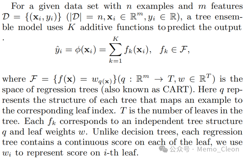
In traditional medical statistics, a sample refers to a part of the observed units randomly drawn from the population. Here, the observed unit is the basic unit of statistical research, that is, an individual/case. However, in the field of machine learning, a sample or instance refers to an individual. In addition, the independent variable in traditional medical statistics is called an attribute or feature in machine learning, while the dependent variable is referred to as a label.

XGBoost Model Theory Introduction and Presentation PPT:

Tianqi Chen, Carlos Guestrin. XGBoost: A Scalable Tree Boosting System.https://github.com/dmlc/xgboost.

Tianqi Chen. Introduction to Boosted Trees.

Tianqi Chen’s PPT 2014 from http://www.washington.edu/

If the network is restricted, it can be downloaded from the address provided in the message.

eXtreme Gradient Boosting Training Function (xgboost package):

xgb.train(params=list(), data, nrounds, watchlist=list(), obj=NULL, feval=NULL, verbose=1, print_every_n=1L, early_stopping_rounds=NULL, maximize=NULL, save_period=NULL, save_name=”xgboost.model”, xgb_model=NULL, callbacks=list(),…)

xgboost(data=NULL, label=NULL, missing=NA, weight=NULL, params=list(), nrounds, verbose=1, print_every_n=1L, early_stopping_rounds=NULL, maximize=NULL, save_period=NULL, save_name=”xgboost.model”, xgb_model=NULL, callbacks=list(),…)

Note: The underscore “_” in the parameters can also be replaced by a dot “.”. xgb.train is a high-level function for training the XGBoost model, while the xgboost function is a simpler wrapper for xgb.train.

Explanation of Various Parameters of the Function:

params: Parameter list. It mainly includes three categories: general parameters, booster parameters, and task parameters. General parameters mainly select the type of base learner, such as tree model or linear model; booster parameters are settings for the selected base learner; and task parameters specify the loss function for training the model and evaluation metrics when using a validation set for model evaluation. For detailed parameter introductions, please refer to the xgboost package help files and XGBoost files [https://xgboost.readthedocs.io/en/latest/parameter.html].

[1] General Parameters:

• booster: Select the base learner; gbtree (default, tree booster. For detailed introduction, see 2.1), gblinear (linear booster. For detailed introduction, see 2.3), dart (boosting tree based on dropout technology from deep neural networks. For detailed introduction, see 2.2);

• device: Specify the running device, CPU (cpu, default) or GPU (cuda). This parameter should be prepared for building complex models that require heavy computation; just building a small clinical model is actually fine with the default;
• verbosity: The level of detail of the information printed by XGBoost. 0 means no printing, 1 prints warning level information, 2 prints info level information, and 3 prints debug level information. The default is 1.
• validate_parameters: When set to true, XGBoost will validate input parameters to check whether parameters are used. If unknown parameters exist, it will issue a warning;
• nthread: Specify the number of parallel threads for XGBoost during runtime, defaulting to the maximum available thread count;
• disable_default_eval_metric: Whether to disable the model’s default evaluation metric. 1 or true indicates disable, default is false.

[2] Booster Parameters:

2.1 gbtree Parameters:

Boosting Tree Ensemble Model and Regression Tree:

Note: The XGBoost ensemble model consists of K additive functions. The expression above represents the estimate of the entire ensemble model for a certain case i. The additive function here is the base learner, and the base learner of XGBoost is commonly a tree model, but it can also be a linear model. When using a tree model, XGBoost is an ensemble algorithm based on regression trees. A single tree is a regression tree rather than a classification tree. Regression trees have the same decision rules as decision trees, but the output of each leaf node in regression trees is a score rather than a label. From this perspective, a regression tree is a function that maps attributes to leaf node score values. Its parameters comprise two parts: one part is the leaf node index function q (structural part), which maps attributes to a specific leaf node, indicating which leaf node the prediction result should belong to; the second part is the output weight value w of that leaf node (weight part), which is the score value mentioned earlier. Regression trees achieve regression, classification, ranking, etc., depending on how the objective function is defined.

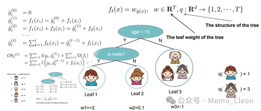
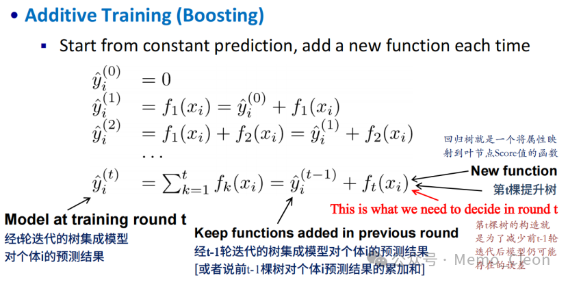
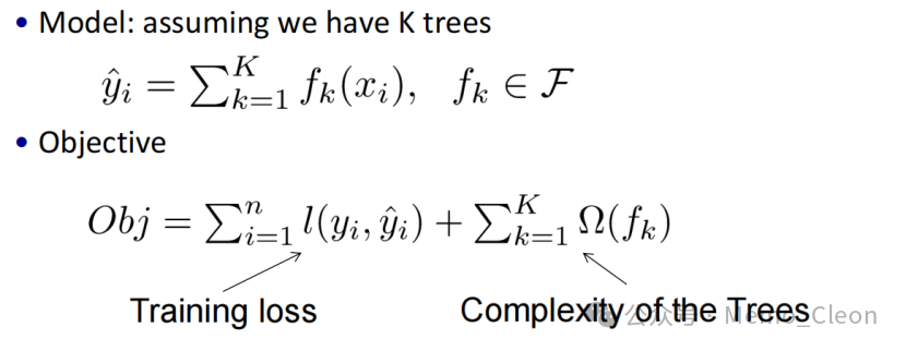
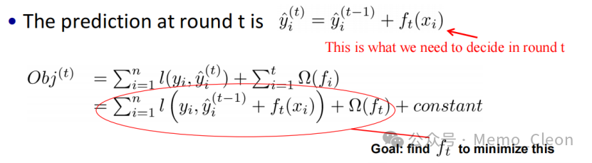
Additive Training (Boosting):

Note:y^{^}_i represents the estimate of the ensemble model after the t-th iteration for individual i, not the prediction result of the t-th tree alone. An XGBoost ensemble model consisting of K trees has undergone K rounds of boosting iterations. In each iteration, a new tree is generated and added to the current model, updating the existing model (i.e., the so-called Additive training or Boosting). The prediction result of the model after t rounds of iteration equals the prediction result of the model after t-1 rounds of iteration plus the output result of the t-th boosting tree. The model after t rounds of iteration (the current model) predicts that the result equals the previous model’s prediction plus the output of the t-th boosting tree. The contribution of each tree (each function) is just an increment, and the final model equals the cumulative sum of the increments from each iteration.

The objective function and model complexity:

Note: The objective function of XGBoost is also the loss function of the entire model, consisting of two parts: the first part is the traditional loss function, which measures the model’s fit to the data, encouraging low bias; the second part is a regularization term that penalizes complex models and encourages simpler models, reducing variance to control the model’s complexity and prevent overfitting.

Each round of iteration aims to find a function that maximally reduces the objective function. The function f_t(x_i) is the t-th boosting tree. When constructing the t-th tree, the models from the previous t-1 rounds are already determined, regardless of their complexity, they are constants. Thus, the constant term in the formula represents the complexity of the ensemble model after t-1 rounds (or the cumulative complexity of the t-1 trees). The formula is simplified through Taylor’s second-order expansion and several transformations (the mathematics involved is beyond the author’s understanding), resulting in the following:

Where g and h represent the first and second derivatives of the loss function at y_i^(t-1), respectively. The gradient is a mathematical concept (a vector whose directional derivative is maximized in that direction, and its magnitude is exactly the maximum directional derivative). The gradient direction of a function is the direction in which the function increases the fastest, while the negative gradient direction is the direction in which the function decreases the fastest.

Definition of tree complexity: γ* number of leaf nodes + 1/2 * α*L1 norm + 1/2 * λ*L2 norm

The more leaf nodes there are, the more splits the tree has, the greater the depth of the tree, and the more complex it is. The complexity of the tree can be measured using the depth of the tree, the number of internal nodes, the number of leaf nodes (T), and the output values of the leaf nodes (W). When the base learner is a CART decision tree, the complexity of XGBoost can be broken down into two parts: the number of leaf nodes T and the output weight values of the leaf nodes w. The number of leaf nodes is assigned a weight γ (this weight is actually the splitting threshold of the node’s splitting point, as will be introduced later), while the weight values of the leaf nodes are regularized.

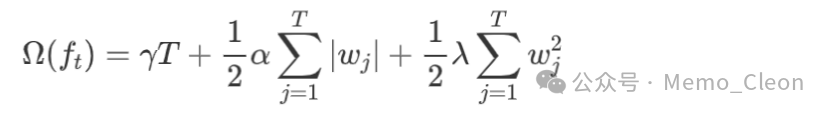
For example, if only the weights are subjected to L2 regularization, the complexity can be simplified to:

Combining the previous definition of the regression tree function, the objective function can evolve into (L2 regularization):

Once the tree structure q(x) is determined, the objective function for this round can be set. This is because it can determine the optimal weight value w* of the leaf node j that minimizes the objective function for this round, as well as the minimum value of the objective function (optimal value):

This is essentially a quadratic equation, seeking the value of w that minimizes Obj and the minimum value. The optimal weight value w* can be obtained through the gradient and Hessian matrix of the loss function. The optimal value of the objective function is also referred to as the structure score, which indicates the maximum reduction in the current objective function when specifying a tree structure. The smaller the value, the better the structure. The fascinating part is that the optimal objective function (structure score) has no relation to the weights.

So how is the tree structure determined? This involves:

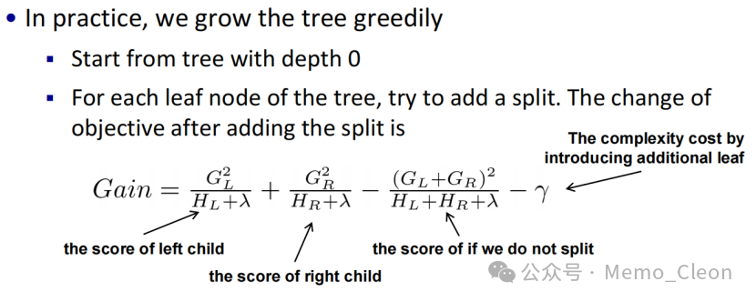
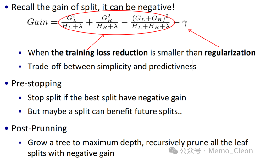
Tree Growth and Pruning:

The growth of the tree mainly involves determining the best splitting attributes and splitting points. In theory, this requires enumerating all possible splitting points on all features (exact greedy algorithm), which is computationally overwhelming. Therefore, other approximate algorithms are often used, such as binning the data first.

For categorical variables, it is recommended to perform one-hot encoding.

The gain from splitting is equal to the structure score after splitting minus the structure score before splitting. The structure score after splitting equals the sum of the structure scores of the left and right subtrees. The larger the Gain value, the more the objective function can be reduced after splitting, which is better:

New splits do not necessarily improve the situation. To optimize this goal (pruning the tree), a penalty term for new leaves is introduced as γ. Whether a new split is reasonable can be assessed by whether it can sufficiently reduce the loss function (structure score). What is considered “sufficient”? This is γ, which can be understood as the threshold for whether a leaf node should be further split. When the reduction in the loss function from the new split (gain) is less than this γ value, the split operation will not be performed. In the definition of tree complexity, it is a weight for the number of leaf nodes (see previous complexity definition). After mathematical transformation, it is assigned a new meaning: the splitting threshold. The optimal γ value is the best split that maximizes the reduction in the loss function.

Key Points of Boosting Tree Algorithm:

The ε in the formula (a variant of ε used in the above image) is the step size of iterative boosting or shrinkage, which is equivalent to the learning rate in GBDT. In the R xgboost function, it is specified by the parameter eta, usually set around 0.1, while in R, the default is 0.3. This is a shrinkage parameter that can be understood as the contribution rate of the output values of the leaves of the current tree (the t-th tree). The introduction of the shrinkage rate reduces the impact of each tree added, leaving more prediction space for subsequent trees, making the boosting process more conservative and robust to prevent model overfitting. A smaller η value means more iterations for the model but requires more computational power and converges more slowly.

• eta: Step size, shrinkage rate, equivalent to the learning rate in GBDT, value range [0,1], default value 0.3. eta is a shrinkage parameter that assigns a weight to the output value of the current tree (the t-th tree) during the t-th iteration.[Refer to the previous introduction of gbtree in the section [Additive Training (Boosting)] and [Key Points of Boosting Tree Algorithm].]

• gamma: Minimum reduction value of the loss function. The minimum reduction value of the loss function required for the leaf nodes to further split is a hyperparameter that measures the complexity of the base learner in the objective function. Its value range is [0, ∞), default value 0. It corresponds to the complexity in the gbtree introduction [Definition of tree complexity: γ * number of leaf nodes + 1/2 * α * L1 norm + 1/2 * λ * L2 norm], which was originally a weight for the number of leaf nodes in the model’s complexity. After several mathematical transformations, it is assigned a new meaning: the splitting threshold. The larger the value, the more conservative the algorithm and the simpler the tree.
• max_depth: Maximum depth of the tree, value range [0, ∞), default 6, where 0 means no depth limit. The larger the value, the more complex the tree, and the more likely it is to overfit.tree_method must be non-zero when set to exact.
• min_child_weight: Minimum threshold for the weight of child nodes, i.e., the minimum value of the case weight (Hessian matrix) on the leaf node. Its value range is [0, ∞), default 1, indicating the minimum sample size required on the leaf node. The larger the value, the less likely it is to form a leaf node, making the algorithm more conservative and the tree simpler. If the weight sum of the cases in a leaf node is less than this value, the branching process will be abandoned. In linear regression tasks (gblinear), this parameter corresponds to the minimum sample size contained in each leaf node, while in gbtree and dart, this parameter is the sum of all second-order derivatives of the samples contained in the leaf node. This parameter is one of the pre-pruning parameters that can help avoid overfitting.
• max_delta_step: Limits the maximum step size of the output value of each tree leaf node, value range [0, ∞), default 0. A value of 0 means no constraint; a positive value makes the algorithm more conservative. Typically, this parameter does not need to be set. It may be useful when conducting logistic regression analysis on highly unbalanced samples. Setting it to 1-10 may help control updates;
• subsample: Sampling ratio of the data, the samples drawn are used for training the model (equivalent to random sampling by rows). Subsampling is performed in each boosting iteration. It is one of the methods to prevent model overfitting, but a value that is too small may lead to underfitting. It is recommended to use this parameter when using the eta parameter and increasing the nrounds value. Its value range is (0, 1], with a default value of 1 indicating that all samples are used for modeling. Setting it to 0.5 means that XGBoost will randomly sample half of the data to train the tree model before growing trees;
• sampling_method: The method of extracting modeling samples from the dataset. By default, uniform means that each case is equally likely to be sampled. It is usually set to subsample >= 0.5 to achieve good results; gradient_based requires the tree_method to be set to hist and the device to be cuda to be available. The probability of each piece of data being sampled is related to the absolute value of the gradient’s regularization, and this method can maintain model accuracy even with subsample values as low as 0.1;
• Column Sampling: colsample_bytree: Specifies the random sampling rate of columns when constructing each tree. A sampling is performed before constructing each tree, and the splitting features of all nodes in the tree are selected from these sampled features (each column corresponds to a feature). Its value range is (0, 1], with a default value of 1 indicating that tree nodes are selected from all features. In addition to randomly selecting modeling features for the entire tree, it is also possible to select splitting features for each level of the tree. The parameter for this is colsample_bylevel, which specifies the sampling ratio of splitting features for each level. Each time the tree reaches a new depth level, a column sampling is performed to select the columns (features) from the column set chosen for the current tree. Additionally, random column sampling can be performed before splitting at each node of the tree to determine the optimal splitting feature; the corresponding parameter is colsample_bynode, which is the feature sampling rate for splitting at each node. Each time a split is performed, a column sampling is performed. The columns are sampled from the column set chosen for the current level. The tree method does not support this parameter when set to exact. These three parameters multiply cumulatively.[Note: Column sampling is a technique in random forests, the purpose of which is to select a portion of all features as the candidate set for node splitting attributes to prevent model overfitting.]
• lambda: L2 regularization weight parameter. [Note: Refer to the comments in the gbtree introduction [Definition of tree complexity] for the λ value in complexity. Its value range is [0, ∞), with a default value of 1, and the larger the value, the more conservative the model.]
• alpha: L1 regularization weight parameter. [Note: Refer to the comments in the gbtree introduction [Definition of tree complexity] for the α value in complexity. Its value range is [0, ∞), with a default value of 0, and the larger the value, the more conservative the model. When α=0 and λ=1, it is equivalent to performing L2 regularization; when λ=0 and α=1, it is equivalent to performing L1 regularization.]
• tree_method: The algorithm for constructing boosting trees in the XGBoost model. Specifically, it refers to the algorithm for selecting the best split points for continuous variables (splitting features) when branching the tree. auto (same as hist, default), exact (exact greedy algorithm that enumerates all possible split points on all features), approx (approximate algorithm that uses quantile sketches and gradient histograms), hist (faster histogram optimized approximate greedy algorithm);
• scale_pos_weight: Controls the weights of negative and positive samples, used in cases of class imbalance. A typical value to consider is the total number of negative samples divided by the total number of positive samples;
• updater: A comma-separated string defining the sequence of tree updaters to run, providing a modular way to build and modify trees. This is a high-level parameter that is usually set automatically based on some other parameters. Available options include grow_colmaker, grow_histmaker, grow_quantile_histmaker, grow_gpu_hist, grow_gpu_approx, sync, refresh, and prune. For details, please refer to the XGBoost files;
• refresh_leaf: A parameter in the updater that indicates whether to refresh the statistics and/or leaf node values based on the current data. Note that this does not execute random subsampling of data rows. The default value is 1, which means updating both leaf node values and node statistics. Setting it to 0 only updates the node statistics;
• process_type: Specifies the type of tree boosting process to execute (create trees, boost trees). The default is the normal boosting process that creates new trees (default), while update indicates that only existing trees will be updated from the current model. In each boosting iteration, a tree is extracted from the initial model, the updater specified in the parameters is run on that tree, and the modified tree is added to the new model. The new model will have the same or fewer trees, depending on the number of boosting iterations executed. Built-in plugins available include refresh and prune, which cannot be used when creating new trees.
• grow_policy: Specifies how new nodes are added. This is only available when the tree_method is set to hist or approx. The default is depthwise, which means splitting closest to the root node. [Note: The closer an attribute is to the root node, the greater the improvement in tree performance measurement.] lossguide performs splits at nodes where the loss function changes the most;
• max_leaves: Maximum number of leaf nodes in the tree. This is available when tree_method is set to exact. The default is 0, indicating no limit;
• max_bin: Maximum number of discrete bins to which continuous variables are split, with a default value of 256. This is only available when tree_method is set to hist or approx. [Note: The greedy algorithm enumerates all features and their splitting points to choose the best one. When the data is large, the computational load is tremendous. In the approximate algorithm, only a portion of candidate split points is selected for enumeration to determine the best split point, making the selection of candidate split points crucial. The primary task is to bin the samples into several groups.]
• num_parallel_tree: Experimental parameter for the number of parallel trees constructed during each boosting iteration. This option supports enhanced random forests, with a default value of 1. A value greater than 1 means that the base learner is no longer a single tree but a random forest. This helps test random forests through XGBoost (the corresponding parameter is set to: colsample_bytree<1, subsample < 1 and round=1);
• monotone_constraints: Monotonicity constraints for variables. A numeric vector consisting of 1, 0, and -1, with a length equal to the number of features in the training data. 1 indicates an increase, -1 indicates a decrease, and 0 indicates no constraint. For details, please refer to the XGBoost files;
• interaction_constraints: A nested vector list of feature indices specifying which features are allowed to interact. Each inner list is a set of indices for features that can interact, e.g., [[0, 1], [2, 3, 4]] indicates that features with column indices 0 and 1 interact, and those with indices 2, 3, and 4 also interact. Note that the feature index values should start from 0 (0 marks the first column), and if there are no interaction terms, this parameter should not be specified.
• multi_strategy: Multi-class outcome data currently supports Python, which is not introduced here.

2.2 gblinear Parameters:

• lambda: L2 regularization weight parameter, with a default value of 0, and the larger the value, the more conservative the model;

• alpha: L1 regularization weight parameter, with a default value of 0, and the larger the value, the more conservative the model;

• updater: The algorithm for fitting linear models. The default is shotgun, a parallel coordinate descent algorithm based on the shotgun algorithm; coord_descent indicates the use of ordinary coordinate descent algorithm.

• feature_selector: Feature selection and ranking method. Available options include cyclic, shuffle, random, greedy, and thrifty;

• top_k: When feature_selector is set to greedy and thrifty, the maximum number of features to be used. The default value is 0, indicating that all features are used.

2.3 dart Parameters:

DART (Dropouts Multiple Additive Regression Trees) is a dropout additive regression tree model.

XGBoost combines a large number of regression trees with a small learning rate, making early-added trees more important than later-added trees. To address overfitting, DART removes some unimportant ordinary trees when constructing new trees to ensure that the contributions of each tree in the final ensemble model are more balanced. DART utilizes the dropout technique from deep neural networks, whereby when computing the gradient that the next tree will fit, only a random subset of the existing ensemble trees is considered. In other words, a portion of trees from the existing ensemble is randomly dropped, and only the remaining trees are used to compute the label (negative gradient) for the next tree. When the new tree is added to the ensemble model, the model results may overshoot, thus DART also performs a normalization step.

Newly constructed trees and dropped trees aim to reduce the gap between the current model and the best predictor. This concept can be difficult to grasp. The dropout action is performed anew in every iteration; trees not used in one iteration may be selected again in the next. The trees randomly discarded in each iteration to compute the label for the next tree are generated using the dropout technique and will also be part of the final ensemble model. After m iterations, when predicting for individual i, the ensemble model still uses m trees, including the trees randomly selected when constructing the m-th tree, the randomly discarded trees, and the m-th tree.

If in the m-th training round, K trees are dropped, the label to be fitted by the m-th tree only uses m-1-K trees (instead of m-1) for estimation. This means that the construction of the m-th tree reduces the potential error still present in the predictions of the m-1 trees. Compared to the m-1 trees model (ordinary boosting model), the m-1-K trees model has a smaller explanation of the outcome, so the label value of the m-th tree is larger. As an additive model, the ensemble model after m iterations includes m trees, comprising the dropped K trees, the m-1-K trees selected for computing the label of the m-th tree, and the m-th tree itself. The ensemble model with m trees will obviously overestimate the outcome, which might explain why literature states that introducing both the new tree and the dropped trees will result in overshooting the target.

The objective function is as follows:

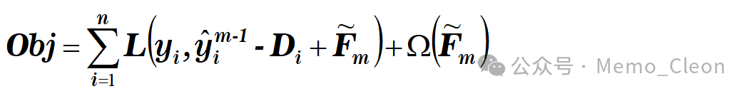
DART can also be seen as a form of regularization, controlling the size of regularization through the number of trees dropped. In special cases, if no trees are dropped, DART is no different from XGBoost; if all trees are dropped, DART is indistinguishable from random forests.

• DART inherits from the gbtree booster, so it supports all parameters of gbtree, such as eta, gamma, max_depth and others. The additional parameters are as follows:

• sample_type: Type of sampling algorithm.uniform (default) means random dropping, i.e., trees to be deleted are chosen with equal probability;weighted means trees are selected for dropping according to their weights;
• normalize_type: Type of normalization algorithm.tree (default) means the new tree’s weight is the same as that of each dropped tree, so α = K/(K+η); forest means the new tree’s weight is equal to the sum of the weights of the dropped trees (forest), so α = 1/(1+η);
• rate_drop: Drop rate, the proportion of trees to be dropped among all trees currently available. Its value range is [0,1], with a default of 0;
• one_drop: Setting this to true means that at least one tree is always dropped during dropout. The default is 0;
• skip_drop: Probability of not executing dropout, with a value range of [0,1], defaulting to 0. If dropout is skipped, the new tree will be added in the same way as in XGBoost.

[3] Task Parameters:

• objective: Specifies the learning task and corresponding objective function. [Note: The objective function here clearly specifies the traditional loss function part in the objective function.] The format is learning task: objective function, where the learning task mainly includes regression, classification, ranking, and survival analysis. Each learning task may have different algorithms, and each algorithm corresponds to different objective functions. For example, reg:squarederror indicates a regression task using squared loss as the loss function, while binary:logistic indicates a binary classification task, where the output of the additive model is a probability (obtained via the sigmoid function) and uses cross-entropy as the loss function. However, the default evaluation metric for the validation set is negative log-likelihood. Many built-in learning tasks: objective functions can be referred to in the xgboost package help files and XGBoost files. In addition to these built-in objective functions, custom functions can also be passed to this parameter via obj.

• base_score: The initial predicted score for all cases, used to set an initial global bias, with a default value of 0.5.

• eval_metric: Evaluation metric for the validation data, allowing multiple metrics to be used.[Note: The explanation in the help file is “evaluation metrics for validation data”. The validation data refers to the dataset used to evaluate model performance, specified by the watchlist. This metric does not affect model training; it is merely an indicator used to evaluate model performance after training is complete.

• seed: Random seed. In R, if not set, it is not defaulted to 0, but is obtained through R’s own RNG engine;

• seed_per_iteration: Determines the seed through the iterator number. The default is false.

data: Training set. xgb.train requires it to be an xgb.DMatrix object.xgboost can be an xgb.DMatrix object, or a matrix, dgCMatrix or local data file;

nrounds: Maximum number of boosting rounds (iterations), which is the number of base learners generated during training;

watchlist: List of DMatrix datasets used to evaluate model performance. The evaluation metrics of these datasets are calculated in each iteration, specified by the parameters eval_metric or feval. The output of this section is stored in the evaluation_log field of the result object.[Note: watchlist is a parameter of the xgb.train function. Setting this parameter in the xgboost function will result in an error (Error in check.custom.obj() : Setting objectives in ‘params’ and ‘obj’ at the same time is not allowed)]

obj: Custom objective function;

feval: Custom evaluation function;

verbose: Displays some information about model performance. 0 means no display, 1 displays model performance information, and 2 displays additional information;

print_every_n: When verbose > 0, prints the model iteration performance information every n iterations. The default value is 1, indicating printing all messages;

early_stopping_rounds: Specifies the number of iterations with no improvement in model performance. If this standard is reached, training will stop. If set to NULL, the early stopping function will not be triggered;

maximize: Indicates whether a higher value of the performance metric is better. [Note: Some evaluation metrics have better performance with lower values, such as mean squared error; while others are better with higher values, such as AUC. Setting this to true indicates that the higher the value (validation score), the better the model performance. If feval and early_stopping_rounds are set, this parameter must also be set;

save_period: Automatically saves the model every few iterations, with 1 indicating once per iteration, and 0 indicating saving at the end;

save_name: Name or path of the model file to be saved periodically;

xgb_model: A previously established model for continued training. It can be an xgb.Booster object or its original data, or the name of a previously saved model;

callbacks: A list of callback functions to execute various tasks during the boosting process. Some callback functions are automatically created based on parameter values, and users can also provide existing or their own callback methods to customize the training process;

label: Specifies the outcome variable. When the data is a local file or an xgb.DMatrix object, this does not need to be provided;

missing: Indicator for missing values, default is NA, which is sometimes represented by 0 or extreme values. This parameter is only used for dense matrix algorithms;

weight: Specifies a vector as the weight for each record.

For categorical variables, the parameters max_cat_to_onehot (whether to use one-hot encoding for variables below the specified threshold) and max_cat_threshold (the maximum number of categories considered for each split) currently support Python.

— END —

@_@