Programmers transitioning to AI are following this account👇👇👇
1 Data Exploration and Preprocessing
1.1 Competition Review
Background
As the world’s largest clean energy source, solar energy is renewable and non-polluting compared to coal and oil; as long as there is sunlight, there is solar energy. Therefore, the utilization of solar energy has been prioritized as a key development project by many countries. However, solar energy has the characteristics of volatility and intermittency. The output power of solar power plants is influenced by various factors, including the performance of photovoltaic panels, meteorological conditions, and operational conditions, making it highly random. This randomness poses significant challenges to the large-scale grid connection of photovoltaic power generation. Accurately predicting the short-term output power of photovoltaic generation and establishing scheduling plans is key to solving this problem. Currently, most photovoltaic power generation prediction technologies focus solely on meteorological conditions and historical data modeling, neglecting the impact of the performance of photovoltaic panels and actual operational conditions on generation efficiency, thus failing to ensure the accuracy of short-term generation power forecasts.
Task
Based on the analysis of photovoltaic generation principles, this study demonstrates the factors affecting photovoltaic output power, such as irradiance and the working temperature of photovoltaic panels. By establishing a prediction model using real-time monitored operational parameters of photovoltaic panels and meteorological parameters, we estimate the instantaneous power generation of photovoltaic power plants, and conduct comparative analysis against actual generation data provided by the DCS system of photovoltaic power plants to verify the practical application value of the model.
Competition code + data + model download link:
Follow the WeChat official account datayx and reply photovoltaic to obtain it.
1.2 Exploratory Data Analysis and Outlier Handling
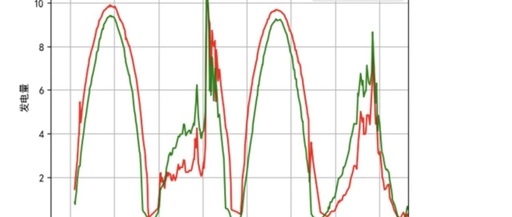
The output power of photovoltaic power plants shows a periodic continuous variable, with a cycle between 180 and 200, which is related to the season. With a total of 17,000 IDs, it can be roughly estimated that there are about 100 cycles. Figure 1 depicts several continuous cycles of power generation. Based on the competition information, we infer that the time span of the training dataset is three months, so we can confirm that one cycle represents one day. However, since we are in the Northern Hemisphere, the duration of sunlight will vary, and as can be seen in the figure, the shape resembles half of a sine function. As shown in Figure 2, the incomplete shape is due to the different weather conditions each day, which leads to changes in light intensity and thus alters the shape of power generation.
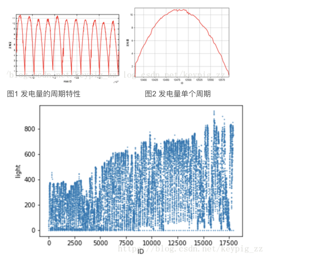
Figure 3: Trend of irradiance variation with ID
After merging the training and testing sets, irradiance and several other features show a roughly continuous variation with ID, and since the ID itself is continuous after merging, there is reason to believe that the test and training sets are randomly sampled from the same dataset. This figure shows that irradiance increases with ID, and the peak value also increases. Since the problem states that these data are from after February 14, we can infer that the photovoltaic power plants in the competition are located in the Northern Hemisphere.
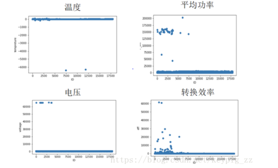
Figure 4 shows the outliers of temperature, average power, voltage A, and conversion efficiency. Figure 4 plots scatter plots for several variables, where we find that these features all contain outliers and anomalies, such as a temperature of -6000, voltage exceeding 60,000, average power exceeding 25,000, wind direction exceeding 360 (which is beyond normal limits), and conversion efficiency anomalies between 10,000 and 30,000. Some outliers appear simultaneously across multiple features.
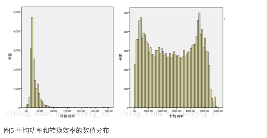
Figure 5 depicts the distribution of values for the features “average power” and “conversion efficiency,” reflecting two different distributions: features with periodic characteristics show a bimodal distribution similar to that of average power, while other features exhibit a normal distribution. Therefore, we determine outliers as data points that exceed three standard deviations from the mean, replacing outliers with the previous value in the column, as the data exhibits continuity and periodicity.
On the other hand, we find that after sunset each day, photovoltaic panels stop generating electricity, and we observe some fixed-value points in power generation, which we did not exploit.
1.3 Correlation Analysis
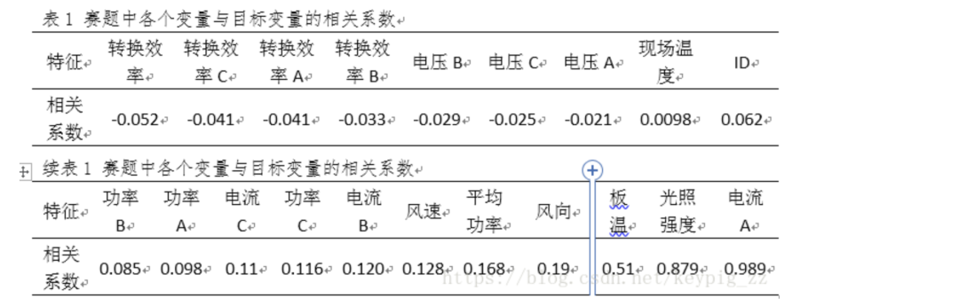
First, we observed the Pearson correlation coefficients between each feature and power generation, with results recorded in Table 1, which can help determine the predictive power of each feature.
Through data visualization, we found that the curve of irradiance/40 closely aligns with the power generation curve, as shown in Figure 6. The curve of average power/480 also closely matches the power generation curve, as shown in Figure 7. The current and power generation are also largely consistent, as shown in Figure 8.
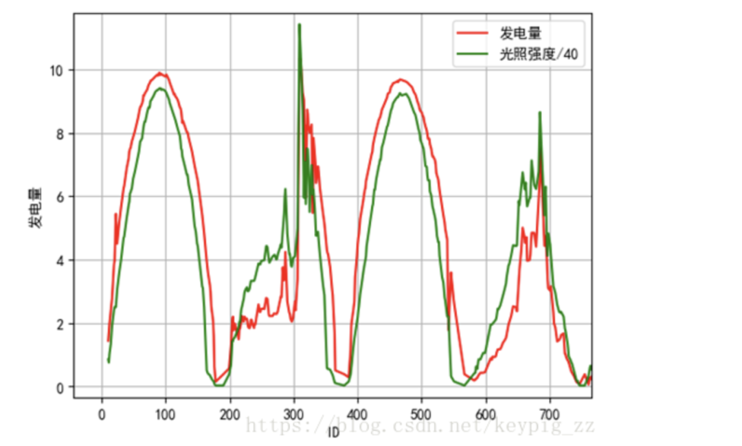
Figure 6: Irradiance/40
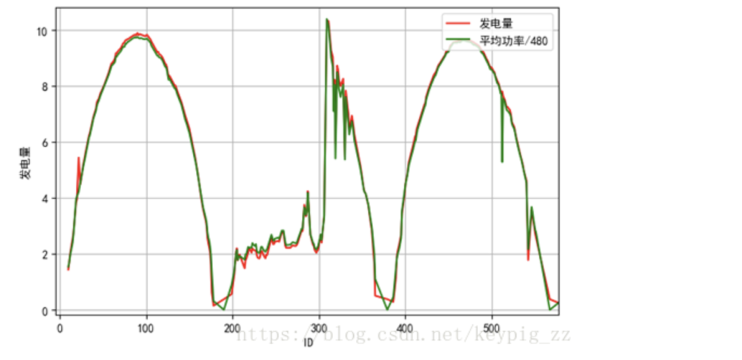
Figure 7: Average Power/480
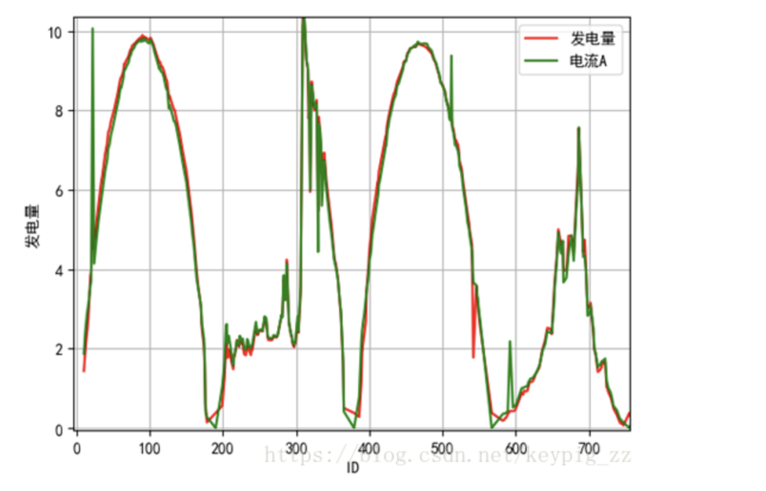 Current A*1.4
The correlation between panel temperature, ambient temperature, and power generation, while not as strong as that of key features, follows a similar trend. Voltage remains stable within a range without showing periodicity, while wind direction is also stable around a certain value, indicating that there has been directional wind over the past three months. Conversion efficiency is generally negatively correlated with power generation, while power generation is highly correlated with irradiance. This indicates that as irradiance increases, conversion efficiency decreases, which literature suggests is due to increased temperature from higher irradiance, and beyond a certain range, higher temperatures reduce efficiency. Figure 8 illustrates the comparison of these three features with power generation.
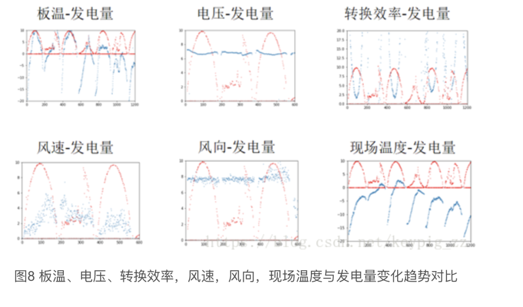
Figure 8: Comparison of panel temperature, voltage, conversion efficiency, wind speed, wind direction, and ambient temperature with power generation trends
2 Feature Engineering
2.1 Features in Photovoltaic Power Generation
Photovoltaic power plants utilize the photovoltaic effect of solar cells to convert light into electrical energy. After analyzing the working principles and power input-output characteristics of photovoltaic systems, we can model the factors affecting photoelectric output and generate new features for photoelectric output prediction using existing data.
Key Feature 1: Forward current of the diode.
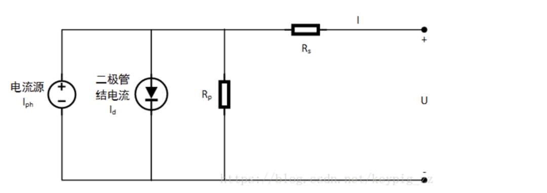
Figure 9: Schematic diagram of the equivalent circuit of photovoltaic power plants
(1) Here, I is the reverse saturation current of the photovoltaic cell diode PN junction.
(2) Key Feature 2: Power from the previous time point.
Since irradiance and the conditions of photovoltaic power plants change relatively slowly over time, using the power from the previous time point as a feature holds certain reference value.
Key Feature 3: Distance to peak within the cycle (dis2peak), average power at the same distance (mean), standard deviation (std).
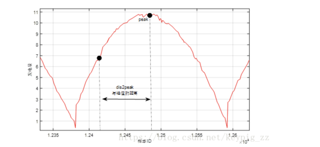
Figure 10: Adding “peak distance” feature based on power generation’s periodic characteristics
Key Feature 4: Temperature difference (panel temperature – ambient temperature).
Panel temperature and ambient temperature influence power generation, and their trends are shown in Figure 11. The difference between the two and power generation also has a strong relationship, as shown in Figure 12.
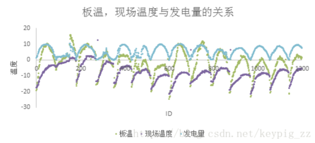
Figure 11: Comparison of panel temperature, ambient temperature, and power generation trends
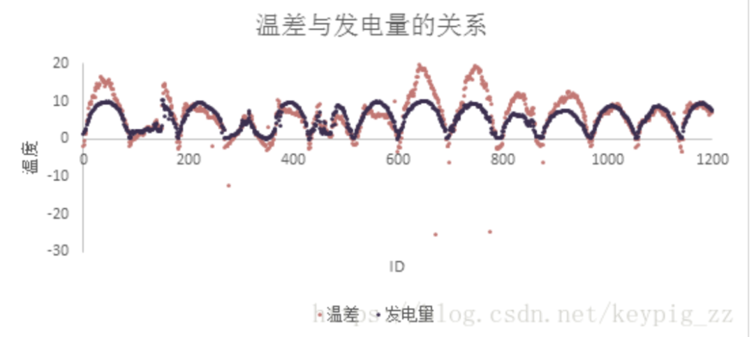
Figure 12: Comparison of temperature difference and power generation trends
Key Feature 5: Voltage A/conversion efficiency = actual irradiance on the panel surface.
Due to the changing angle of sunlight throughout the day, the provided irradiance cannot directly reflect the irradiance on the panel surface. Through literature review, the calculation method for conversion efficiency is photovoltaic panel output power/irradiance power, where the output power of the photovoltaic panel is represented by voltage A. Given the known conversion efficiency, voltage A/conversion efficiency can represent the actual irradiance on the panel surface.
Key Feature 6: Power/wind speed at the node.
Through the paper “Analysis of Wind Speed, Power, and Power Curve of Wind Turbines,” we know that wind speed can influence the output power of generators, thus further affecting power generation. Therefore, we constructed the feature power/wind speed at each node.
2.2 High-Order Environmental Features
In special engineering, one idea is to utilize combinations of existing features to compute their high-order features. Through feature selection, we found that the second-order interaction terms between environmental factors such as ‘panel temperature’, ‘ambient temperature’, ‘irradiance’, ‘wind speed’, and ‘wind direction’ can provide better predictive performance.
2.3 Feature Selection
In the competition, our basic approach was to use different features for different models. This is because during the competition, we found that features that were very effective on one model did not necessarily yield good results on another model.
Additionally, we employed the “forward feature selection” method during the competition. The basic process of this method is to first select the parameter with the best predictive performance, then continue to select one feature from the remaining features to form a feature set that maximizes the score. This process continues until the maximum number of features or the entire feature set is reached.
Figure 13 illustrates the scoring situation as features are added during the forward feature selection process. The testing process used the LightGBM model (detailed parameters can be found in the submitted code).
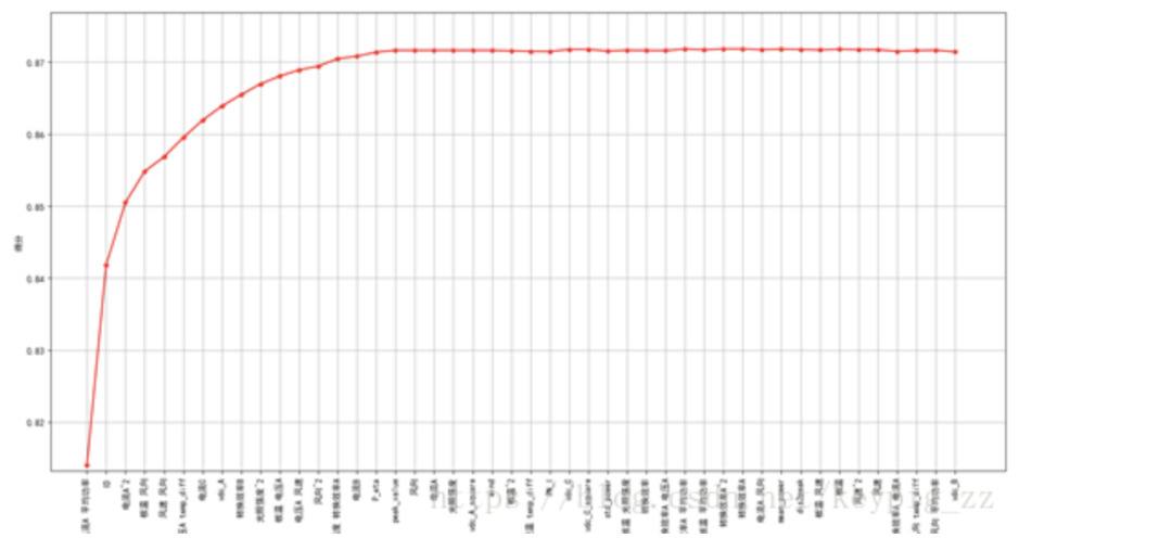
Figure 13: Scoring curve of forward feature selection
3 Model Construction and Tuning
3.1 Overall Structure of Prediction Model
This is a regression prediction problem for a continuous target variable, and many models can effectively solve such problems. However, there are differences in principles and results between different models. In the competition, we adopted the idea of Stacking, integrating the three models: LightGBM, XGBoost, and LSTM. The first two can be regarded as tree models, while LSTM is a neural network model. The principles of these two types of models differ significantly, and the results produced are less correlated, which is beneficial for improving prediction accuracy. The specific model structure is illustrated in Figure 14.
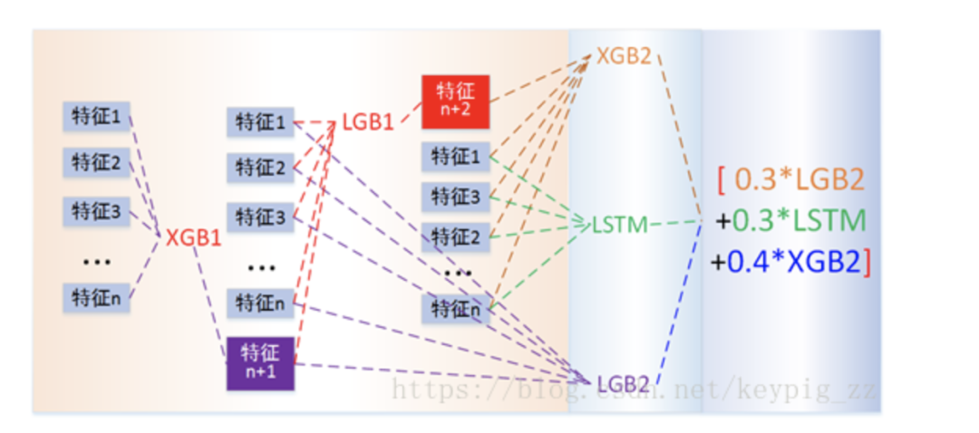
Figure 14: Overall structure of the prediction model
We used Xgboost_1 to learn feature combination F1, obtaining the prediction results of Xgboost_1 (including predictions for both the training and testing sets). This result will serve as a new feature, added to feature combinations F2 and F3, respectively, as input features for the second layer LightGBM_1 and LightGBM_2. The result of LightGBM_1 will again serve as a new feature, added to feature combination F4, serving as input for the third layer Xgboost_2, while the third layer also includes an LSTM model, which is trained using feature combination F5. The results of the second layer LightGBM_2 will be combined with the prediction results of the third layer Xgboost_2 and LSTM through weighted integration to produce the final result.
3.2 Construction and Tuning Based on LightGBM and XGBoost
A significant issue in this problem is overfitting. We found that the model performed excellently on the training samples but poorly on the validation and test datasets. After implementing effective methods such as feature and sample sampling into training, reducing tree depth, and adjusting regularization parameters, we discovered that the following innovative methods could further reduce overfitting.
Reusing some features.
In the Light GBM model, we executed a duplication of environmental features (panel temperature, ambient temperature, irradiance, wind speed, wind direction), meaning these features appeared twice during training. The results showed that the training set error was nearly identical, but the validation errors for both the online and offline datasets were smaller. This indicates that using duplicate features reduced the degree of overfitting, enhancing the model’s generalization and predictive performance.
Comparing the training curves of the training set with and without duplicate features, as shown in Figure 15, it is evident that the validation errors of the model with duplicate features are smaller than those of the model without duplicate features, while the training errors of both are nearly the same.
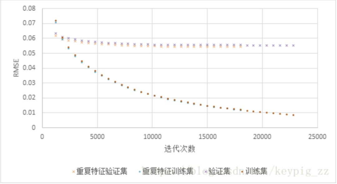
Figure 15: Cross-validation error curve with duplicate features
Many literature and experiments indicate that removing highly correlated features during feature selection is beneficial. However, in this case, we found that while duplicate features are highly correlated with existing features, this approach can improve predictive accuracy. We believe this may be related to the higher probability of sampling duplicate features when individual tree models sample features.
Whether this finding is universal requires experimental validation on other datasets.
Predicting after each fold of cross-validation.
Parameter tuning for single models significantly affects model performance. We utilized grid search and cross-validation methods to obtain the optimal parameter combinations within specified parameter ranges. Upon determining the parameters, we applied cross-validation again during training for single models. This allows for comparison of different model effects, and during 4-fold cross-validation, after each fold of training, we predict the test set using the model obtained from that fold of cross-validation. Specifically, for the Xgboost model, after 4-fold cross-validation, we obtain four different “Xgboost models,” using these four models to predict the test set separately. The final prediction result of Xgboost is the average of the four prediction results. This process can be viewed as a sampling of the training set. The final result of Xgboost is essentially a fusion of the results from four sub-models. Sampling and fusion can reduce overfitting, and we found that such processing improves prediction accuracy for this problem.
Each single model uses different features.
Each single model (including LSTM) shares 90% of the features in common, while approximately 10% of the features are unique to each model. By increasing the differentiation between models in this way, we reduce dependence on a single feature combination, enhancing the generalization ability of the models, and achieving better fusion results.
3.3 Construction and Tuning Based on LSTM
Long Short-Term Memory (LSTM) networks are a type of recurrent neural network capable of addressing issues arising from long-term information. In LSTM, the cell is the basic unit, and Figure 16 illustrates the basic unit of LSTM as well as the network formed by connecting these basic units.
Within a cell, there is a structure called a “gate,” as shown in Figure 17. The Sigmoid function outputs a value between 0 and 1, which, when multiplied by the output of the previous cell, determines how much information can pass through.
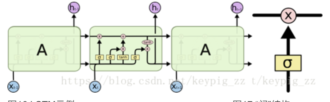
Figure 17: The “gate” structure
In this competition, we used a single-layer LSTM network containing 200 units, structured as shown in Figure 18.
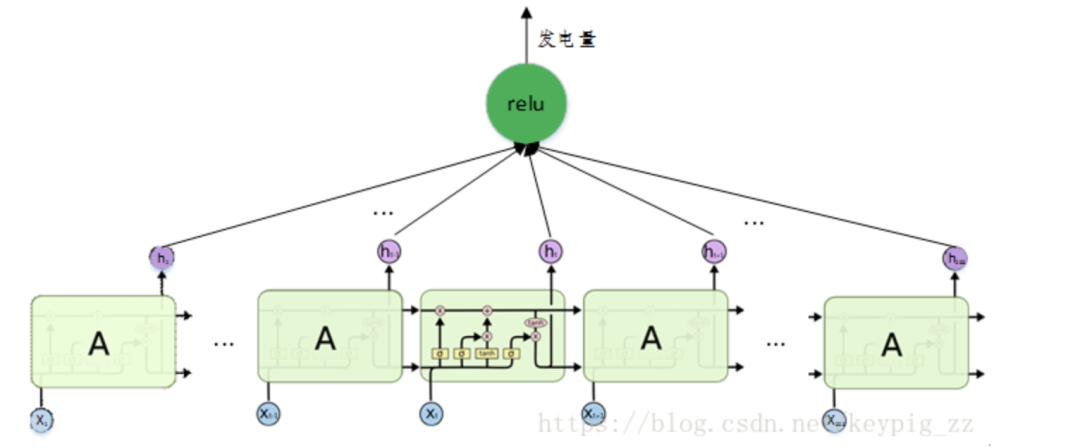
Figure 18: LSTM network structure used in the competition
The error curves for training and validation of the network are shown in Figure 19.
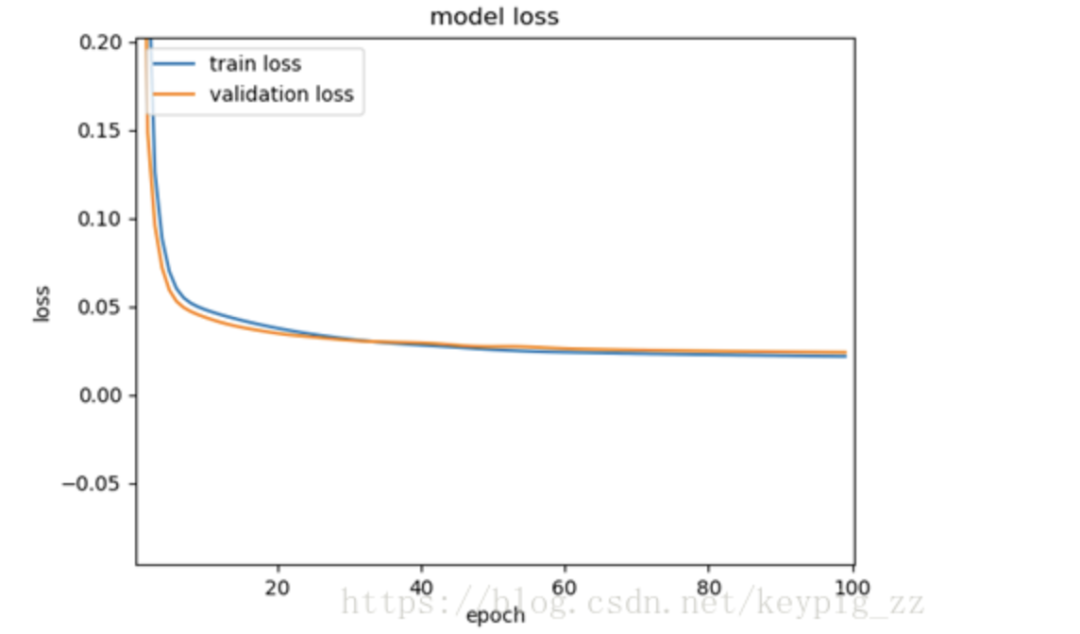
Figure 19: LSTM training error graph
3.4 Model Fusion and Summary
Model fusion is a highly effective technique that can enhance regression or classification accuracy in most machine learning tasks. Different models’ result files can be fused directly, or the prediction results of one model can be used as features for training another model, leading to new prediction results. In this competition, we comprehensively utilized both fusion methods.
Different types of models learn training principles differently, and the knowledge they acquire varies. In this competition, through submissions during the competition, we observed that tree models (XGBoost and LightGBM) and LSTM single models exhibit strong learning capabilities. After linear fusion of several models, the predictive capability is further enhanced. The fused model achieved the best results in the competition.
4 Summary and Outlook
We would like to express our gratitude to the State Power Investment Corporation and DF platform for hosting such a competition. Throughout the competition, we gained friendships and knowledge, honed our skills, and broadened our horizons.
During the competition, we believe the following factors contributed to our continuous self-improvement and good results.
From a team perspective, we consistently trusted each other, communicated diligently, collaborated effectively, and did not give up easily. These team factors supported us throughout the competition, whether we were lagging behind or leading the rankings, as we continually searched for new literature and breakthrough ideas. It was through repeated attempts that our features became more effective, our models more refined, and ultimately yielded high scores.
From a technical standpoint, the following aspects were key:
Reasonable Data Preprocessing
We observed outliers in the data and applied the same outlier repair method (previous value filling) to both training and testing data.
Efficient Feature Construction and Selection
We constructed powerful features such as diode node flow and conversion efficiency calculations by reviewing literature in the field of photovoltaic power generation. Additionally, we employed a more scientific feature selection method—forward feature selection.
Carefully Designed Fusion Model
The fusion model constructed based on LightGBM, XGBoost, and LSTM can leverage the complementary advantages of the three models while reducing the impact of overfitting.