Author丨Tian Yu Su
Zhihu Column丨Machine Learning
Link丨https://zhuanlan.zhihu.com/p/27234078
1. Introduction
This sharing mainly focuses on the translation, understanding, and integration of two English documents on the Word2Vec model, both of which introduce the Skip-Gram model in Word2Vec. The next column article will implement the basic version of the Word2Vec Skip-Gram model using TensorFlow, so this article serves as a theoretical foundation. Please refer to the original English documents:– Word2Vec Tutorial – The Skip-Gram Model– Word2Vec (Part 1): NLP With Deep Learning with Tensorflow (Skip-gram)
2. What is Word2Vec and Embeddings?
Word2Vec is a model that learns semantic knowledge from a large amount of text corpus in an unsupervised manner, and it is widely used in Natural Language Processing (NLP). How does it help us with NLP? Word2Vec represents the semantic information of words through word vectors by learning from text, meaning that semantically similar words are close to each other in an embedding space. Embedding is essentially a mapping that translates words from their original space into a new multi-dimensional space, embedding the original word space into a new one. Intuitively, the word “cat” is semantically close to “kitten”, while “dog” and “kitten” are not as close, and “iphone” is even further away from “kitten”. By learning this numerical representation of words in the vocabulary (i.e., converting words into word vectors), we can perform vector operations based on these numbers to derive interesting conclusions. For example, if we perform the operation: kitten – cat + dog on the word vectors, the resulting embedded vector will be very close to the word vector for “puppy”.
3. Part One
Model
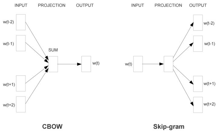
In the Word2Vec model, there are mainly two models: Skip-Gram and CBOW. Intuitively, Skip-Gram predicts the context given an input word. CBOW predicts the input word given the context. This article will only explain the Skip-Gram model.
The basic form of the Skip-Gram model is very simple. To clarify the model, we first look at the most general basic model of Word2Vec (hereafter, all references to Word2Vec denote the Skip-Gram model).
The Word2Vec model is actually divided into two parts: the first part is establishing the model, and the second part is obtaining the embedded word vectors through the model. The entire modeling process of Word2Vec is actually very similar to the idea of an auto-encoder, where a neural network is constructed based on training data. Once the model is trained, we do not use this trained model for new tasks; what we really need are the parameters learned from the training data, such as the weight matrix of the hidden layer—what we actually aim to learn in Word2Vec are the “word vectors”.
In the process of modeling based on training data, we call it the “Fake Task”, implying that modeling is not our final goal.
The method mentioned above is actually seen in unsupervised feature learning, most commonly in auto-encoders: encoding the input in the hidden layer, compressing it, and then decoding it back to the initial state in the output layer. After training, we will “cut off” the output layer and only keep the hidden layer.
The Fake Task As mentioned above, the true purpose of training the model is to obtain the hidden layer weights learned based on the training data. To get these weights, we first need to build a complete neural network as our “Fake Task”. Later we will return to see how we indirectly obtain these word vectors through the “Fake Task”. Next, let’s see how to train our neural network. Suppose we have a sentence “The dog barked at the mailman“.
-
First, we select a word from the middle of the sentence as our input word; for example, we choose “dog” as the input word;
-
After having the input word, we define a parameter called skip_window, which represents the number of words we select from one side (left or right) of the current input word. If we set skip_window=2, then the words we finally obtain in the window (including the input word) will be [‘The’, ‘dog’, ‘barked’, ‘at’]. skip_window=2 means selecting 2 words to the left and 2 words to the right of the input word, so the total window size span=2*2=4. Another parameter called num_skips represents how many different words we select from the entire window as our output word. When skip_window=2 and num_skips=2, we will get two sets of training data in the form of (input word, output word), namely (‘dog’, ‘barked’), (‘dog’, ‘the’).
-
The neural network will output a probability distribution based on these training data, which represents the likelihood of each word in our vocabulary being the output word. This statement may sound complex, so let’s look at an example. In the second step, when we set skip_window and num_skips=2, we obtained two sets of training data. If we take one set of data (‘dog’, ‘barked’) to train the neural network, then the model will inform us of the probability of each word in the vocabulary being “barked” based on this training sample.
The output probability of the model indicates how likely each word in our vocabulary is to appear with the input word. For example, if we input the word “Soviet” into the neural network model, then in the final output probability, related words like “Union” and “Russia” will have a much higher probability than unrelated words like “watermelon” and “kangaroo”. This is because “Union” and “Russia” are more likely to appear in the context of “Soviet”.
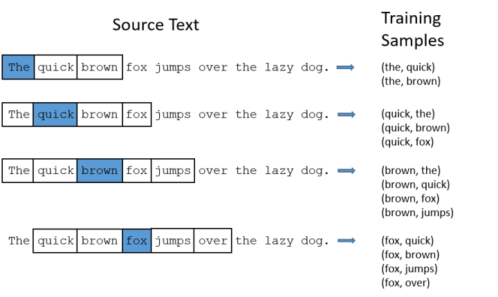
We will train the neural network by inputting paired words from the text to calculate the probabilities mentioned above. The following figure shows some examples of our training samples. We take the sentence “The quick brown fox jumps over lazy dog“, and set our window size to 2 (window_size=2), meaning we only select two words before and after the input word to combine with the input word. In the figure below, blue represents the input word, and the words within the box are those located in the window.
Our model will learn statistical results from the frequency of occurrence of each pair of words. For example, our neural network might see more training sample pairs like (“Soviet”, “Union”) and very few combinations like (“Soviet”, “Sasquatch”). Therefore, after training, when we input the word “Soviet”, the output probabilities for “Union” or “Russia” will be higher than for “Sasquatch”.
Model Details
How do we represent these words?
First, we know that neural networks can only accept numerical input, so we cannot input a word string directly; therefore, we need a method to represent these words. The most common method is to build our own vocabulary based on the training documents and then perform one-hot encoding on the words.
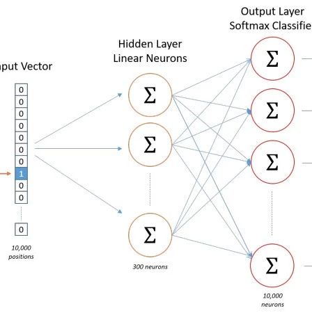
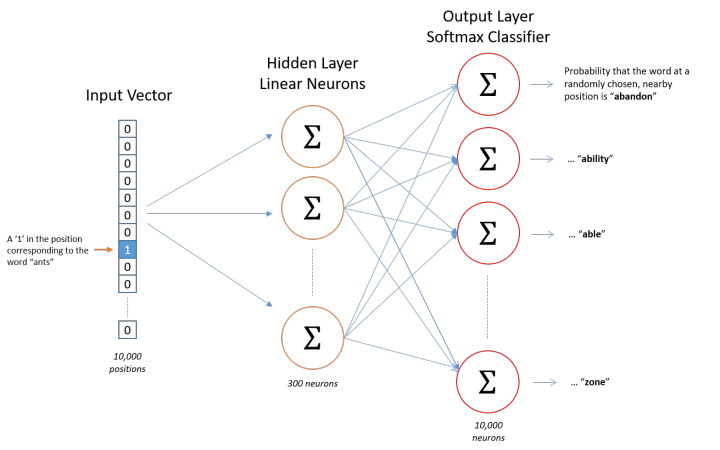
Assuming we extract 10,000 unique words from our training documents to form a vocabulary. We perform one-hot encoding on these 10,000 words, resulting in each word being represented as a 10,000-dimensional vector, where each dimension has a value of either 0 or 1. If the word “ants” appears in the third position in the vocabulary, then the vector for “ants” will be a 10,000-dimensional vector with a value of 1 in the third dimension and 0 in all others (ants = [0,0,1,0,…,0]).
Using the previous example, for the sentence “The dog barked at the mailman”, we can construct a vocabulary of size 5 (ignoring case and punctuation): (“the”, “dog”, “barked”, “at”, “mailman”), and we number the words in this vocabulary from 0-4. Thus, “dog” can be represented as a 5-dimensional vector [0,1,0,0,0].
If the input to the model is a 10,000-dimensional vector, then the output is also a 10,000-dimensional vector (the size of the vocabulary), which contains 10,000 probabilities, each representing the probability of the current word being the output word in the input sample.
The following diagram shows the structure of our neural network:

The hidden layer does not use any activation function, but the output layer uses softmax. We train the neural network based on paired words, where the training samples are word pairs in the form of (input word, output word), and both input words and output words are one-hot encoded vectors. The final output of the model is a probability distribution.
Hidden Layer Now that we have discussed the encoding of words and the selection of training samples, let’s look at our hidden layer. If we want to represent a word with 300 features (i.e., each word can be represented as a 300-dimensional vector), then the weight matrix of the hidden layer should have 10,000 rows and 300 columns (the hidden layer has 300 nodes).
Google’s latest model trained on the Google News dataset uses word vectors with 300 features. The dimensionality of word vectors is a hyperparameter that can be adjusted (in Python’s gensim package, the default word vector size for the Word2Vec interface is 100, and window_size is 5).
Looking at the images below, the left and right images represent the input layer to the hidden layer weight matrix from different angles. In the left image, each column represents a 10,000-dimensional word vector and the weight vector connecting to a single neuron in the hidden layer. In the right image, each row actually represents the word vector for each word.
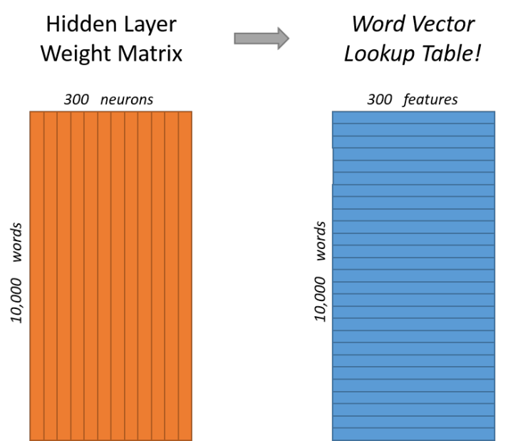
Thus, our ultimate goal is to learn this hidden layer weight matrix.
Now let’s continue training our model based on its definition.
As mentioned earlier, both input words and output words will undergo one-hot encoding. Upon careful consideration, after one-hot encoding, most dimensions of our input are 0 (in fact, only one position is 1), so this vector is quite sparse. What will this result in? If we multiply a 1 x 10,000 vector with a 10,000 x 300 matrix, it will consume a significant amount of computational resources. For efficient computation, it will only select the rows in the matrix corresponding to the indices where the vector has a dimension value of 1 (this statement may sound complex), and the diagram will clarify it.
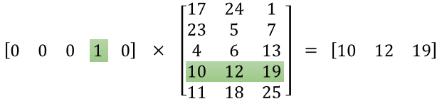
Let’s look at the matrix operation in the figure above. On the left are 1 x 5 and 5 x 3 matrices, and the result should be a 1 x 3 matrix. According to the rules of matrix multiplication, the first row and first column element of the result is 0*17+0*23+0*4+1*10+0*11=10; similarly, the other two elements are 12 and 19. If the 10,000-dimensional matrix is computed in this way, it is quite inefficient.
To compute efficiently, matrix multiplication will not be performed in this sparse state. The result of the matrix computation is actually the weights corresponding to the indices in the vector where the value is 1. In the above example, the left vector has a value of 1 in the 3rd dimension (0-based index), so the computation result is the 3rd row of the matrix (0-based index)—[10, 12, 19]. Thus, the hidden layer weight matrix in the model becomes a “lookup table”, where during matrix computation, it directly retrieves those weight values corresponding to the dimensions where the input vector has a value of 1. The output of the hidden layer is the “embedded word vectors” for each input word.
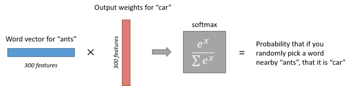
Output Layer
After the calculation in the hidden layer of the neural network, the word “ants” will transform from a 1 x 10,000 vector to a 1 x 300 vector, which will then be input into the output layer. The output layer is a softmax regression classifier, where each node will output a value between 0 and 1 (probability), and the sum of the probabilities from all output layer neurons equals 1. Below is an example of the calculation for the training sample (input word: “ants”, output word: “car”).
Intuitive Understanding
Next, we will engage in some intuitive thinking. If two different words have very similar “contexts” (meaning the window words are quite similar, such as “Kitty climbed the tree” and “Cat climbed the tree”), then through our model training, the embedded vectors for these two words will be very similar. For example, for the samples (Kitty, climbed) and (Cat, climbed), with the same output but different inputs, after repeated training, the embeddings for Cat and Kitty will get closer! This is because they share a similar loss, which will update to bring Cat and Kitty’s embeddings closer!
So what does it mean for two words to have similar “contexts”? For instance, for synonyms like “intelligent” and “smart”, we believe these two words should have the same “context”. Similarly, related words like “engine” and “transmission” might also share similar contexts. In fact, this method can also assist in stemming, as the neural network will learn similar word vectors for “ant” and “ants”.
Stemming is the process of removing affixes to obtain the root of a word.
This part concludes here, and the next part will delve into how to efficiently train on the Skip-Gram model.

Recommended Reading:
Practical | Pytorch BiLSTM + CRF for NER
How to evaluate the fastText algorithm proposed by the author of Word2Vec? Does deep learning have no advantages in simple tasks like text classification?
From Word2Vec to Bert, discussing the evolution of word vectors (Part 1)