
Reprinted from: Machine Learning Beginner
0. Introduction
Word embeddings refer to a set of language models and representation learning techniques in Natural Language Processing (NLP). Conceptually, it involves embedding a high-dimensional space of the number of words into a much lower-dimensional continuous vector space, where each word or phrase is mapped to a vector in the real number domain.
This article explainsthe basics of word embeddings and Word2vec.
Author of this article:
jalammar (https://jalammar.github.io)
Translation:
Huang Haiguang (https://github.com/fengdu78)
The code in this article can be downloaded from GitHub:
https://github.com/fengdu78/Data-Science-Notes/tree/master/8.deep-learning/word2vec
Illustration of Word2vec
Start of the main text
I find the concept of embeddings to be one of the most fascinating ideas in machine learning. If you have ever used Siri, Google Assistant, Alexa, Google Translate, or even the next word prediction feature on your smartphone keyboard, you have likely benefited from this idea, which has become central to NLP models. Over the past few decades, there has been significant development in neural models using embedding techniques (recent developments include contextual embeddings in cutting-edge models like BERT and GPT-2).
Since 2013, Word2vec has been an effective method for creating word embeddings. In addition to the method of embedding words, some of its concepts have proven effective in creating recommendation engines and understanding sequential data in non-linguistic tasks. Companies like Airbnb, Alibaba, Spotify, and Anghami have taken this excellent tool from the NLP world and put it into production, supporting novel recommendation engines.
We will discuss the concept of embeddings and the mechanism for generating embeddings using Word2vec.
Let’s start with an example to understand how vectors can represent things.
Did you know that a list of five numbers (vectors) can represent your personality?
Personality Embedding: What’s Your Personality Like?
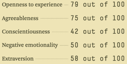
Using a range from 0 to 100 to represent your personality (where 0 is the most introverted and 100 is the most extroverted).
The Big Five personality traits test asks you a list of questions and scores you on many aspects, one of which is introversion/extroversion.
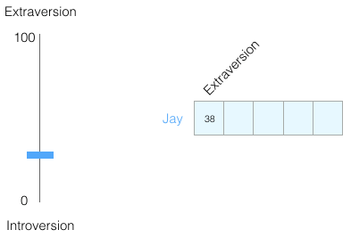
Now let’s switch the range to -1 to 1:
Understanding a person requires more than one-dimensional information, so let’s add another dimension – the score of another trait in the test.
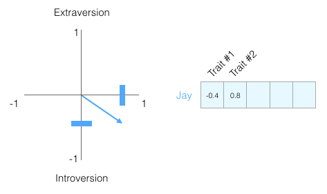
You may not know what each dimension represents, but you can still gain a lot of useful information from the vector representation of a person’s personality.
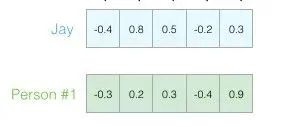
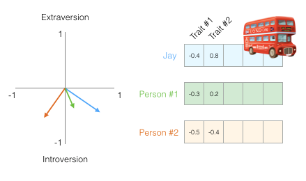
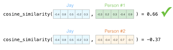
Now we can say that this vector partially represents my personality. The usefulness of this representation becomes apparent when you want to compare two other people with me. In the next figure, which of the two individuals is more like me?
When dealing with vectors, a common method for calculating similarity scores is cosine similarity:
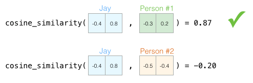
Person 1 has a high cosine similarity score with me, so our personalities are quite similar.
However, two dimensions are still not enough to capture sufficient information about different populations. Decades of psychological research have studied five main traits (and many sub-traits). So we use all five dimensions in our comparisons:
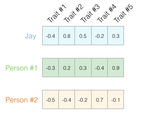
We cannot plot five dimensions in two-dimensional space, which is a common challenge in machine learning; we often need to think in higher-dimensional spaces. But the advantage is that cosine similarity still works. It applies to any number of dimensions:
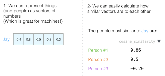
The two central ideas of embeddings:
-
We can represent people (things) as vectors of numbers. -
We can easily calculate the relationships between similar vectors.
Word Embeddings
We import GloVe vectors trained on Wikipedia
import gensim
import gensim.downloader as api
model = api.load('glove-wiki-gigaword-50')
Word embedding representation of the word "king":model["king"]array([ 0.50451 , 0.68607 , -0.59517 , -0.022801, 0.60046 , -0.13498 ,
-0.08813 , 0.47377 , -0.61798 , -0.31012 , -0.076666, 1.493 ,
-0.034189, -0.98173 , 0.68229 , 0.81722 , -0.51874 , -0.31503 ,
-0.55809 , 0.66421 , 0.1961 , -0.13495 , -0.11476 , -0.30344 ,
0.41177 , -2.223 , -1.0756 , -1.0783 , -0.34354 , 0.33505 ,
1.9927 , -0.04234 , -0.64319 , 0.71125 , 0.49159 , 0.16754 ,
0.34344 , -0.25663 , -0.8523 , 0.1661 , 0.40102 , 1.1685 ,
-1.0137 , -0.21585 , -0.15155 , 0.78321 , -0.91241 , -1.6106 ,
-0.64426 , -0.51042 ], dtype=float32)View the most similar words to “king”
model.most_similar("king")[('prince', 0.8236179351806641),
('queen', 0.7839042544364929),
('ii', 0.7746230363845825),
('emperor', 0.7736247181892395),
('son', 0.766719400882721),
('uncle', 0.7627150416374207),
('kingdom', 0.7542160749435425),
('throne', 0.7539913654327393),
('brother', 0.7492411136627197),
('ruler', 0.7434253096580505)]This is a list of 50 numbers, and we cannot clearly articulate what each value represents. We line up all these numbers so we can compare them with other word vectors. Let’s color-code the cells based on their values (red if close to 2, white if close to 0, and blue if close to -2)
import seaborn as sns
import matplotlib.pyplot as plt
import numpy as np

plt.figure(figsize=(15, 1))
sns.heatmap([model["king"]],
            xticklabels=False,
            yticklabels=False,
            cbar=False,
            vmin=-2,
            vmax=2,
            linewidths=0.7)
plt.show()
We will ignore the numbers and only look at colors to indicate the values of the cells, comparing “King” with other words:
plt.figure(figsize=(15, 4))
sns.heatmap([
    model["king"],
    model["man"],
    model["woman"],
    model["king"] - model["man"] + model["woman"],
    model["queen"],
],
            cbar=True,
            xticklabels=False,
            yticklabels=False,
            linewidths=1)
plt.show()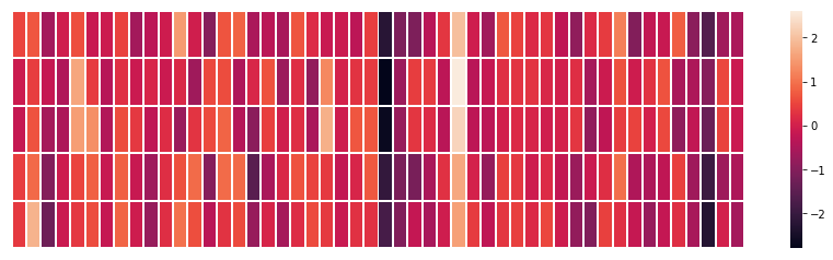
Notice how “man” and “woman” are more similar to each other than either is to “king”? This tells you something. These vector representations capture information/meaning/associations of these words.
Here’s another example list (find similar colored columns by scanning vertically):
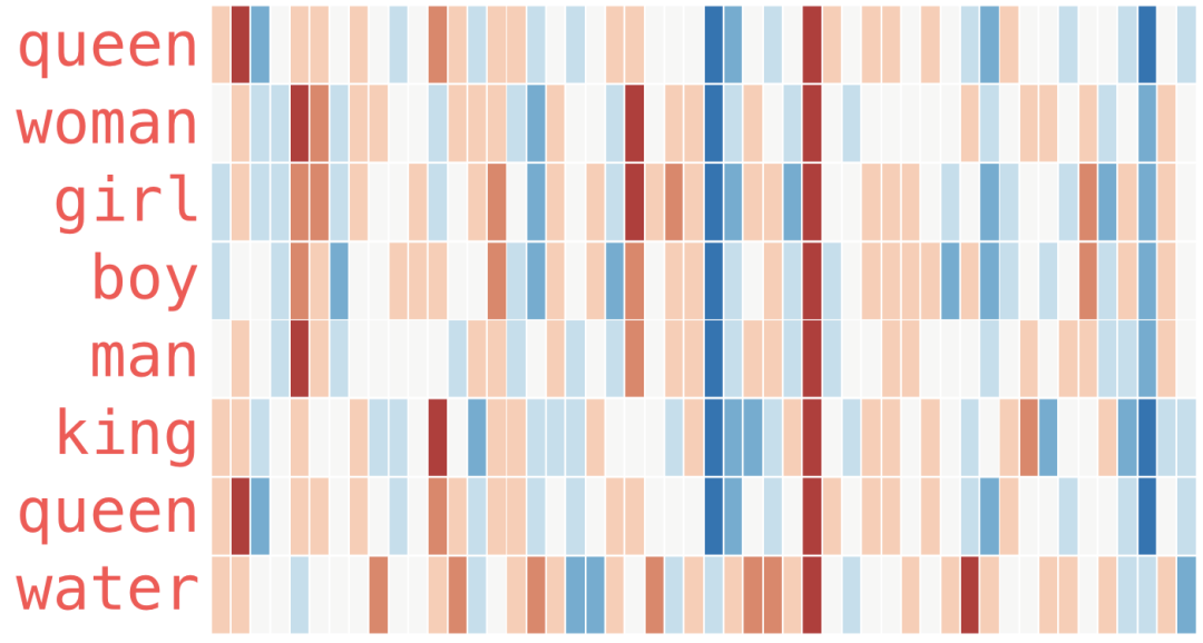
Several points to note:
-
All these different words have a straight red column. They are similar in this dimension (we don’t know what each dimension code is). -
You can see how “woman” and “girl” are similar in many ways, just like “man” and “boy”. -
“Boy” and “girl” also have similarities to each other but differ from “woman” or “man”. Could this write a fuzzy concept of youth? Perhaps. -
All words except the last one represent people. I added the object “water” to show the differences between categories. For example, you can see the blue column continues downward and stops before embedding “water”. -
It’s evident that “king” and “queen” are similar to each other and different from everyone else.
Analogy
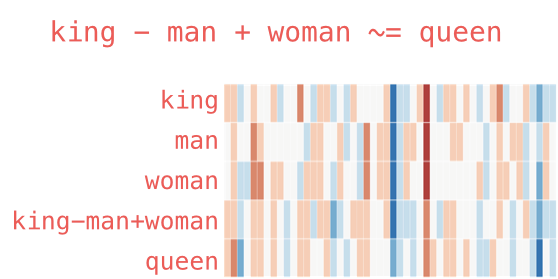
We can add and subtract word embeddings to obtain interesting results, the most famous example being the formula: “king” – “man” + “woman”:
model.most_similar(positive=["king","woman"],negative=["man"])[('queen', 0.8523603677749634),
('throne', 0.7664334177970886),
('prince', 0.759214460849762),
('daughter', 0.7473883032798767),
('elizabeth', 0.7460220456123352),
('princess', 0.7424569725990295),
('kingdom', 0.7337411642074585),
('monarch', 0.7214490175247192),
('eldest', 0.7184861898422241),
('widow', 0.7099430561065674)]We can visualize this analogy as before:
Language Modeling
If you want an example of an NLP application, one of the best examples would be the next word (token) prediction feature of smartphone keyboards. This is a feature used hundreds of times a day by billions of people.
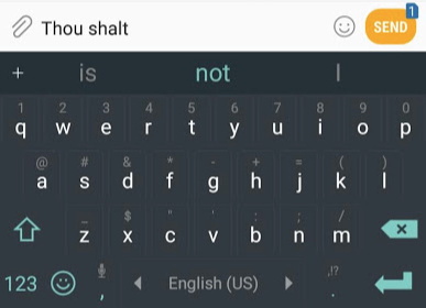
The next word (token) prediction is a task that can be solved by language models. A language model can take a list of words (say two words) and attempt to predict the word that follows them.
In the above screenshot, we can view the model as taking these two green words (thou shalt) and returning a list of suggestions (“not” is the word with the highest probability):
We can think of the model as this black box:
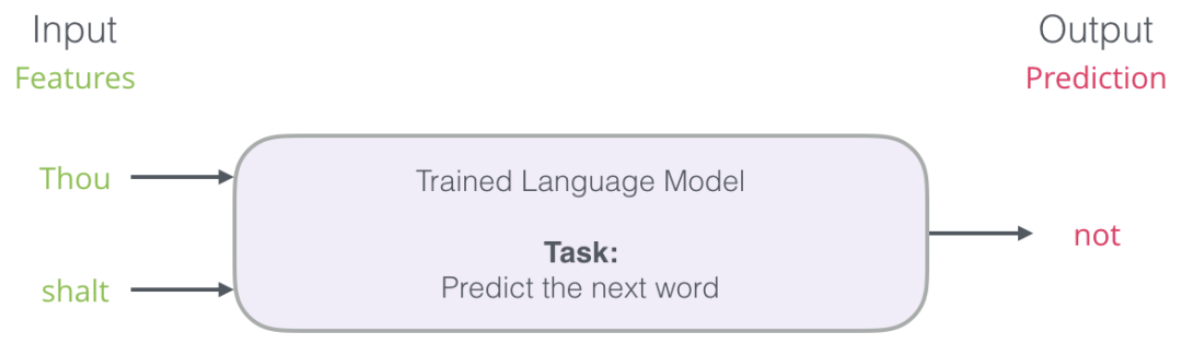
But in reality, the model does not output just one word. It actually outputs probability scores for all the words it knows (the model’s “vocabulary”, which can range from several thousand to over a hundred thousand words). The application must then find the word with the highest score and present it to the user.
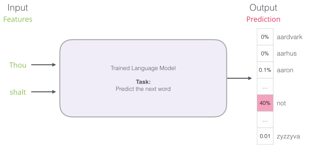
Figure: The output of a neural language model is the probability scores of all the words the model knows. We refer to the probabilities here as percentages, for example, a probability of 40% will be represented as 0.4 in the output vector.
After training, early neural language models (Bengio 2003) calculated predictions in three steps:
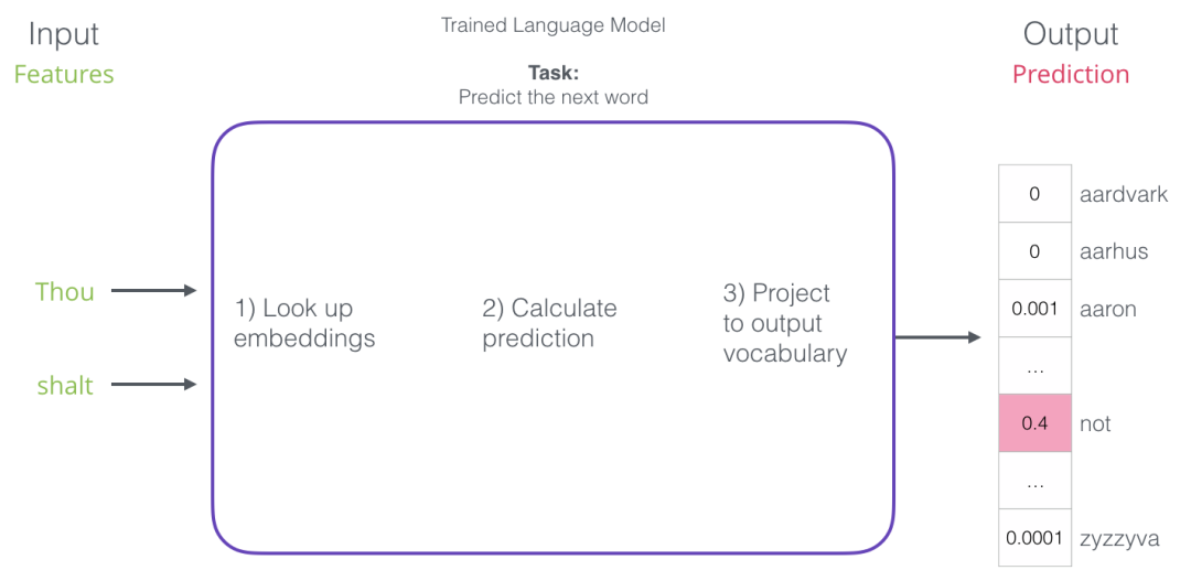
When discussing embeddings, the first step is the most relevant to us. One of the results of the training process is this matrix that contains the embeddings for every word in our vocabulary. During prediction time, we only look up the embeddings for the input words and use them to calculate the predictions:
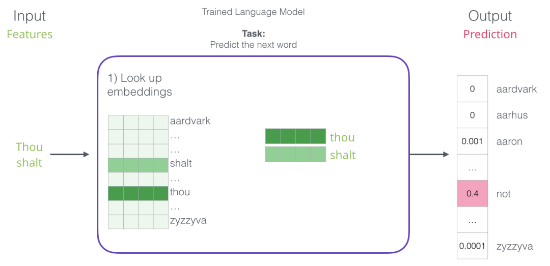
Now let’s turn to the training process to understand how the embedding matrix works.
Training Language Models
Compared to most other machine learning models, language models have a huge advantage. That is: all of our books, articles, Wikipedia content, and other forms of massive text data can serve as training data. In contrast, many other machine learning models require manually designed features and specially collected data.
Words are embedded by looking at the other words that tend to appear next to them. The mechanism works like this:
-
We obtain a large amount of text data (for example, all Wikipedia articles). Then -
We have a window (say three words) that we slide across all the text. -
The sliding window generates training samples for our model.

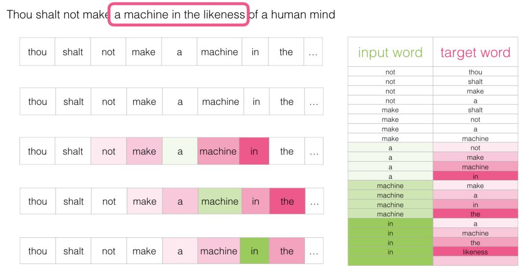
As this window slides over the text, we (virtually) generate a dataset for training the model. To accurately see how this is done, let’s look at how the sliding window processes this phrase:
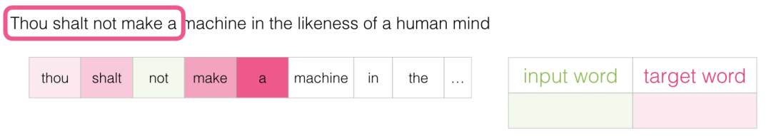
When we start, the window is on the first three words of the sentence:
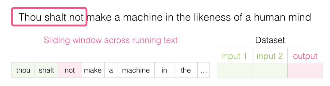
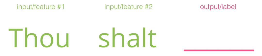
We take the first two words as features and the third word as the label:
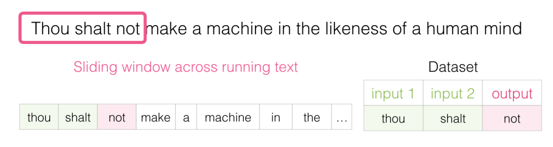
We have now generated the first sample in the dataset, which we can later use to train the language model.
Then we slide the window to the next position and create the second sample:
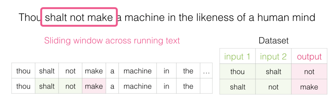
Now we have generated the second example.
Soon we will have a larger dataset with different word pairs appearing:
In practice, the model is often trained as we slide the window. However, I find it clearer logically to separate the “dataset generation” phase from the training phase. Besides the neural network-based language modeling approaches, a technique known as N-gram is often used to train language models.
To understand how this transition from N-gram to neural models reflects real-world products, I recommend reading this blog post from 2015 that introduces their neural language model and compares it with the previous N-gram models.
Looking Both Ways
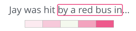
Given the content before your sentence, fill in the blanks:

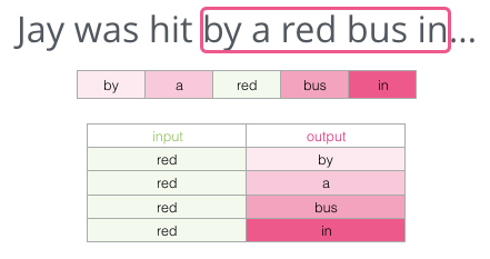
The background I give you here is the five words before the blank (and the previously mentioned “bus”). I believe most people would guess that the word in the blank would be “bus”. However, if I give you another piece of information: the sentence after the blank, would that change your answer?

This completely changes what should be left in the blank. The word “red” is now the most likely to fill the blank. What we learn from this is that the words before and after specific words both have informational value. It turns out that considering both directions (the words to the left and right of the word we are guessing) allows word embeddings to perform better.
Let’s see how we can adjust the way we train our models to address this issue.
Skipgram
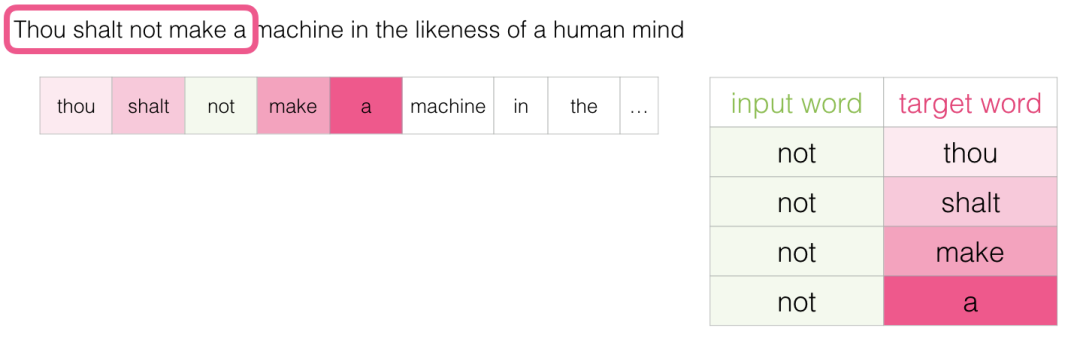
We can look at not only the two words before the target word but also the two words after it.

If we do this, the dataset we actually build and train our model on will look like this:
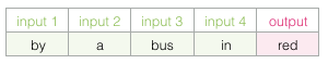
This is called the continuous bag-of-words structure and is described in one of the Word2vec papers.
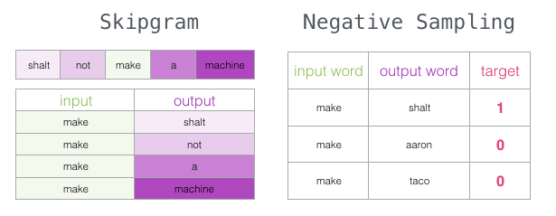
Another structure is slightly different from the continuous bag-of-words structure but can also show good results. This structure tries to use the current word to guess the neighboring words rather than guessing a word based on its context (the words before and after it). We can visualize it as a sliding window over the training text as follows:
This method is called the skipgram architecture. We can visualize the sliding window as follows:
This adds these four samples to our training dataset:
Then we slide the window to the next position:
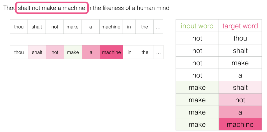
This will produce our next four samples:
Revisiting the Training Process
Now that we have extracted our skipgram training dataset from the existing running text, let’s see how we use it to train a basic neural language model that predicts adjacent words.
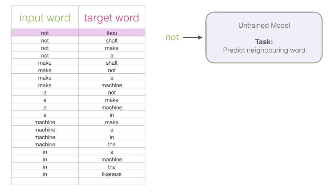
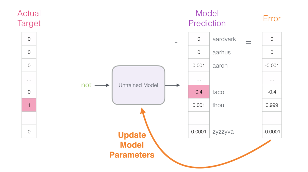
We start with the first sample in the dataset. We provide the features to the untrained model and ask it to predict a suitable adjacent word.
The model performs three steps and outputs a prediction vector (probability distribution for each word in its vocabulary). Since the model is untrained, the predictions at this stage are certainly incorrect. But that’s okay. We know what it should guess: the label/output cell in the row we are currently using to train the model:
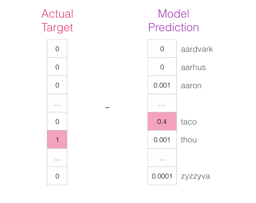
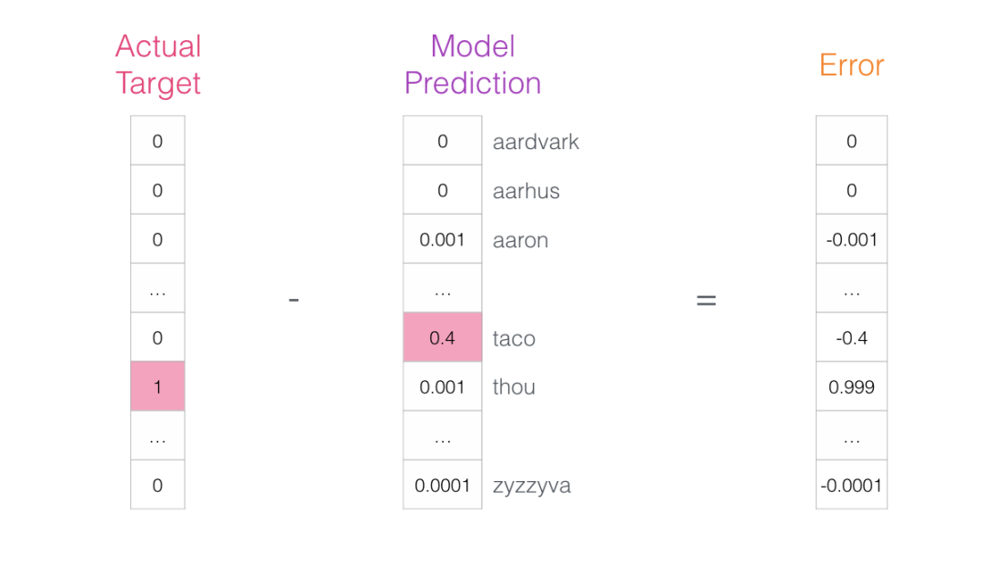
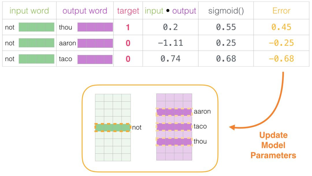
This error vector can now be used to update the model so that the next time “not” is input, the model is more likely to guess “thou”.
This is the first step of training. We continue with the next sample in the dataset using the same process, then the next sample, until we cover all samples in the dataset. This completes one epoch of training. We continue training for multiple epochs, and then we have a trained model from which we can extract the embedding matrix and use it for any other application.
While this deepens our understanding of the process, it is still not the actual training process of Word2vec.
Negative Sampling
Recall how this neural language model calculates its predictions in three steps:
From a computational perspective, the third step is very resource-intensive: especially since we will do this for each training sample in the dataset (likely tens of millions of times). We need to do something to improve efficiency.
One approach is to split the target into two steps:
-
Generate high-quality word embeddings (don’t worry about predicting the next word). -
Use these high-quality embeddings to train the language model (perform next word prediction).
We will focus on step 1, as we focus on embeddings. To generate high-quality embeddings using high-performance models, we can switch the task of the model from predicting adjacent words:
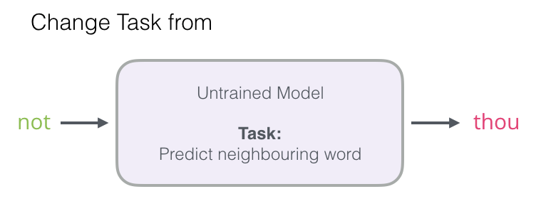
And switch it to a model that takes input and output words and outputs a score indicating whether they are neighbors (0 means “not neighbors”, 1 means “neighbors”).
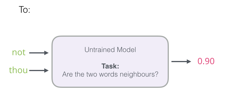
This simple change switches the model we need from a neural network to a logistic regression model: thus it becomes simpler and faster to compute.
This change requires us to switch the structure of the dataset – the labels are now a new column with values of 0 or 1. They will all be 1 because all the words we add are neighbors.
Now it can be computed at incredible speeds – processing millions of examples in a matter of minutes. But we need to close a loophole. If all our examples are positive (target: 1), we open the possibility for our smart model to always return 1 – achieving 100% accuracy but learning nothing and generating garbage embeddings.
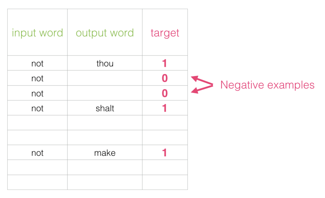
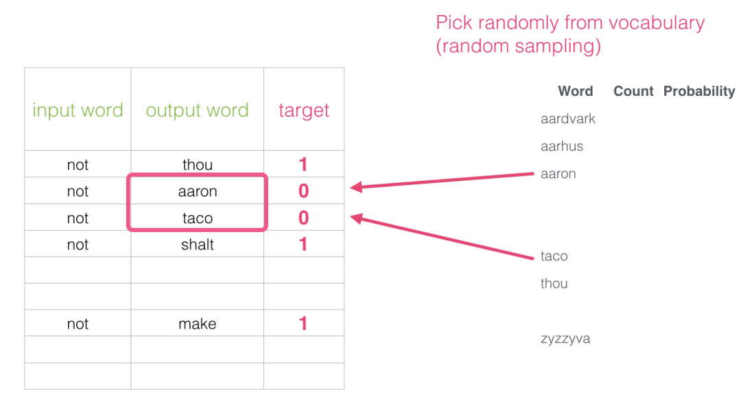
The inspiration for this idea comes from noise-contrastive estimation. We contrast the actual signal (positive examples of adjacent words) with noise (randomly chosen words that are not neighbors). This is a huge trade-off in computational and statistical efficiency.
Skipgram with Negative Sampling (SGNS)
We have now introduced two core ideas in Word2vec:
skipgramandnegative sampling.
Word2vec Training Process
Now that we have established the two central ideas of skipgram and negative sampling, we can continue to examine the actual Word2vec training process in detail.
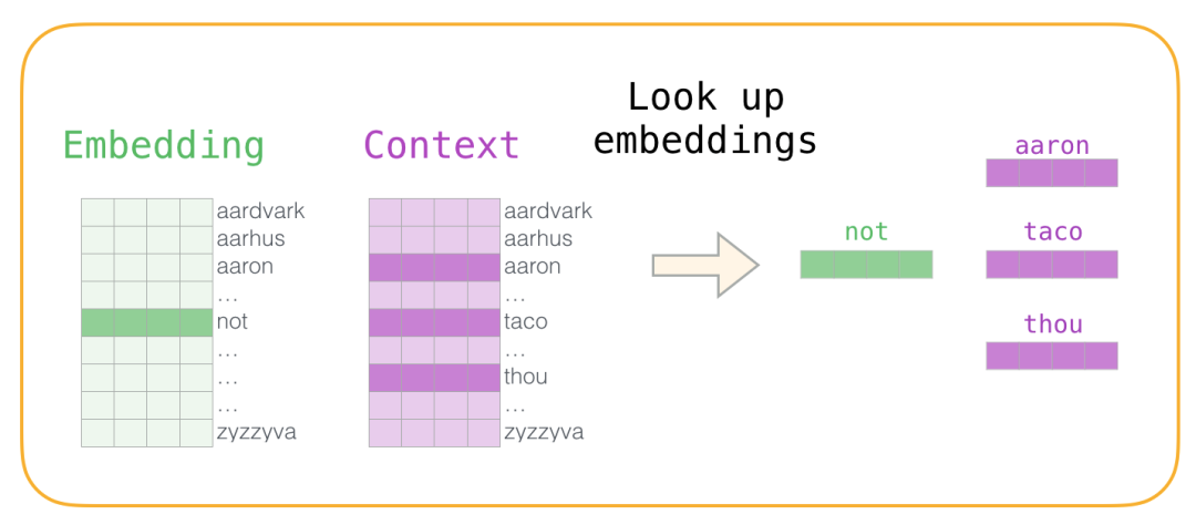
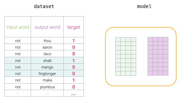
Before the training process begins, we preprocess the text that we are training the model on. At this step, we determine the size of the vocabulary (which we call vocab_size, say, consider it as 10,000) and which words belong to it. At the beginning of the training phase, we create two matrices – Embedding matrix and Context matrix. These two matrices embed each word in our vocabulary (this vocab_size is one of their dimensions). The second dimension is the length of the embedding we want at each time (commonly embedding_size – 300 is a common value, but the example earlier in this article was 50).
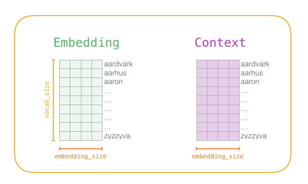
At the beginning of the training process, we initialize these matrices with random values. Then we start the training process. In each training step, we take a positive sample and its related negative samples. Let’s take a look at our first set:
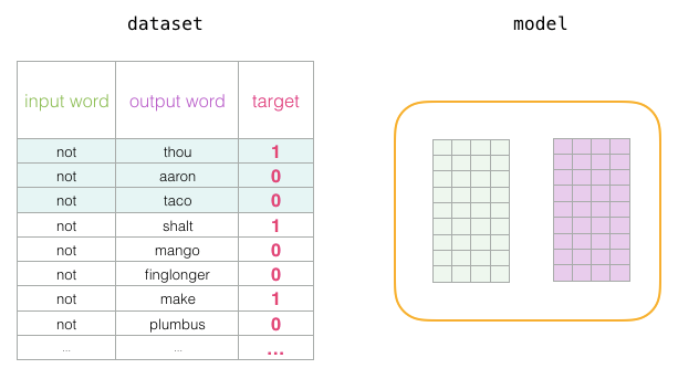
Now we have four words: the input word not and the output/context words: (thou the actual neighbor), aaron, and taco (negative samples). We look up their embeddings – for the input word, we check the Embedding matrix. For the context words, we check the Context matrix (even though both matrices embed each word in our vocabulary).
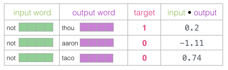
Then, we calculate the dot product of the input embedding with each context embedding. In each case, a number is produced that indicates the similarity of the input and context embeddings.
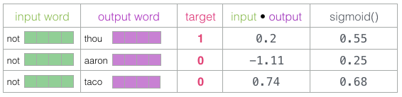
Now we need a method to transform these scores into something that looks like probabilities: we use the sigmoid function to convert the scores into values between 0 and 1.
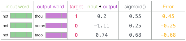
Now we can view the output of the sigmoid operation as the model’s output for these samples. You can see taco scored higher than aaron, and still had the lowest score before and after the sigmoid operation. Now that the untrained model has made predictions and we see we have an actual target label to compare, let’s calculate the error in the model’s predictions. To do this, we simply subtract the sigmoid score from the target label.
Window Size and Number of Negative Samples
Two key hyperparameters in the Word2vec training process are the window size and the number of negative samples.
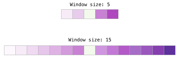
Different window sizes can better serve different tasks.
A heuristic approach is to use smaller window embeddings (2-15), where a high similarity score between two embeddings indicates that these words are interchangeable (note that if we only look at surrounding words, antonyms can often be interchangeable – for example, good and bad often appear in similar contexts).
Using larger window embeddings (15-50 or even more) yields embeddings where similarity better indicates word relevance. In practice, you often need to provide annotated guidance for the embedding process to bring useful similarity for your task.
Gensim defaults the window size to 5 (the input word itself plus the two words before and after the input word).
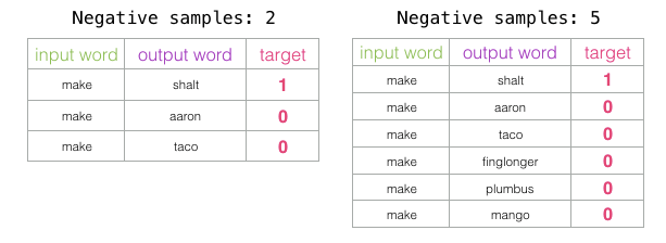
The number of negative samples is another factor in the training process. The original paper suggested a number of negative samples between 5-20. It also noted that when you have a sufficiently large dataset, 2-5 seems to be sufficient. Gensim defaults to 5 negative samples.
Conclusion
I hope you now have a better understanding of word embeddings and the Word2vec algorithm. I also hope that now when you read a paper mentioning “skip gram with negative sampling” (SGNS), you will have a better grasp of these concepts.
Author of this article: jalammar (https://twitter.com/jalammar).
References and Further Reading
-
Distributed Representations of Words and Phrases and their Compositionality [pdf]
-
Efficient Estimation of Word Representations in Vector Space [pdf]
-
A Neural Probabilistic Language Model [pdf]
-
Speech and Language Processing by Dan Jurafsky and James H. Martin is a leading resource for NLP. Word2vec is tackled in Chapter 6.
-
Neural Network Methods in Natural Language Processing by Yoav Goldberg is a great read for neural NLP topics.
-
Chris McCormick has written some great blog posts about Word2vec. He also just released The Inner Workings of word2vec, an E-book focused on the internals of word2vec.
-
Want to read the code? Here are two options:
-
Gensim’s python implementation of word2vec
-
Mikolov’s original implementation in C – better yet, this version with detailed comments from Chris McCormick.
-
Evaluating distributional models of compositional semantics
-
On word embeddings, part 2
-
Dune
Download 1: Four-piece set
Reply "four-piece set" in the backend of the public account for machine learning algorithms and natural language processing to get the learning materials for TensorFlow, Pytorch, machine learning, and deep learning!


Download 2: Repository address sharing
Reply "code" in the backend of the public account for machine learning algorithms and natural language processing to get 195 NAACL + 295 ACL2019 papers with open-source code. The open-source address is as follows: https://github.com/yizhen20133868/NLP-Conferences-Code

Heavy! The machine learning algorithms and natural language processing exchange group has been officially established! There are a lot of resources in the group, and everyone is welcome to join the group for learning!

Additional benefits! Qiu Xipeng's deep learning and neural networks, official Chinese tutorials for Pytorch, data analysis using Python, machine learning learning notes, official Chinese documentation for pandas, effective java (Chinese version), and other 20 welfare resources

How to get: After entering the group, click on the group announcement to get the download link
Note: Please modify the remarks when adding to [School/Company + Name + Direction]
For example - Harbin Institute of Technology + Zhang San + Dialogue System.
The account owner, please consciously avoid. Thank you!


Recommended reading:
12 Golden Rules for Solving the NER Problem in Industry

Three Steps to Master the Core of Machine Learning: Matrix Derivation

Distillation Techniques in Neural Networks, Starting with Softmax