Big Data DigestProduced by
Author: Jay Alammar
Embedding is one of the most fascinating ideas in machine learning. If you have ever used Siri, Google Assistant, Alexa, Google Translate, or even your smartphone keyboard for next word prediction, you have likely benefited from this idea that has become central to natural language processing models.
Over the past few decades, embedding techniques have seen significant development in neural network models. Recently, this development includes contextual embeddings that led to cutting-edge models like BERT and GPT2.
BERT:
https://jalammar.github.io/illustrated-bert/
Word2Vec is an effective method for creating word embeddings, existing since 2013. However, beyond being a method for word embeddings, some of its concepts have proven effective in creating recommendation engines and understanding temporal data in business, non-linguistic tasks. Companies like Airbnb, Alibaba, and Spotify have drawn inspiration from the field of NLP and applied it to their products, supporting new types of recommendation engines.
In this article, we will discuss the concept of embeddings and the mechanism of generating embeddings using Word2Vec. Let’s start with an example to familiarize ourselves with using vectors to represent things. Did you know that your personality can be represented by just a list of five numbers (vectors)?
Personality Embedding: What Kind of Person Are You?
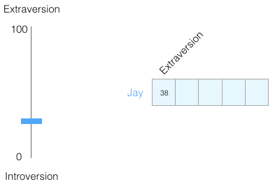
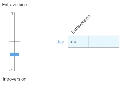
How do you represent how introverted/extroverted you are on a scale from 0 to 100 (where 0 is the most introverted and 100 is the most extroverted)? Have you ever taken personality tests like MBTI or the Big Five personality traits test? If you haven’t, these tests ask you a series of questions and then score you on many dimensions, one of which is introversion/extroversion.
Example results from the Big Five personality traits test. It can tell you a lot about yourself and has predictive power in academic, personality, and career success. You can find the test results here.
Assuming my introversion/extroversion score is 38/100. We can plot it this way:
Let’s narrow the range to -1 to 1:
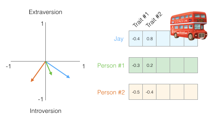
When you only know this one piece of information, how well do you think you understand this person? Not very well. People are complex. Let’s add another test score as a new dimension.

We can represent the two dimensions as a point on a graph, or as a vector from the origin to that point. We have great tools to handle the incoming vectors.
I’ve hidden the personality traits we are plotting so that you gradually get used to extracting valuable information from a vector representation of a personality without knowing what each dimension represents.
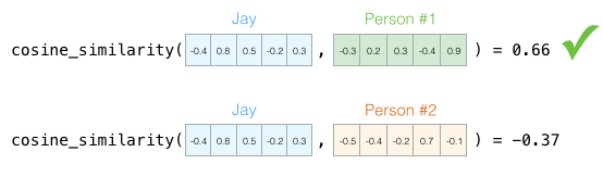
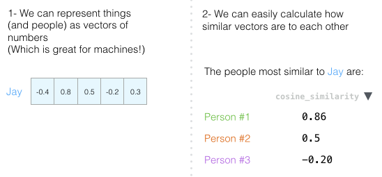
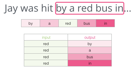
We can now say this vector partially represents my personality. This representation becomes useful when you want to compare two other people to me. Suppose I get hit by a bus, and I need to be replaced by someone with a similar personality; which of the two people in the image below is more like me?
When processing vectors, a common method for calculating similarity scores is cosine similarity:
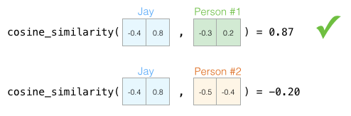
Person 1 is more similar to me in personality. Vectors pointing in the same direction (length also matters) have a higher cosine similarity.
Once again, two dimensions are still not enough to capture sufficient information about different populations. Psychology has identified five main personality traits (along with a large number of subtraits), so let’s use all five dimensions for comparison:
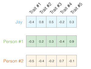
The problem with using five dimensions is that we can no longer neatly plot small arrows on a two-dimensional plane. This is a common issue in machine learning, where we often need to think in higher-dimensional spaces. Fortunately, cosine similarity still works; it applies to any number of dimensions:
Cosine similarity works for any number of dimensions. These scores are better than the previous ones because they are calculated based on higher-dimensional comparisons.
At the end of this section, I would like to propose two central ideas:
1. We can represent people and things as algebraic vectors (which is great for machines!).
2. We can easily compute the relationships between similar vectors.
Word Embedding
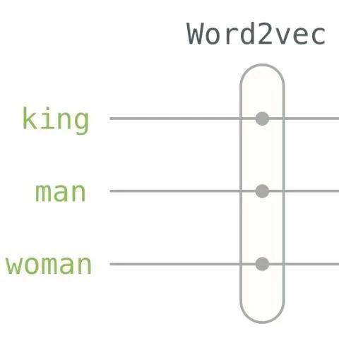
With the understanding from the above, let’s continue to look at examples of trained word vectors (also known as word embeddings) and explore some of their interesting properties.
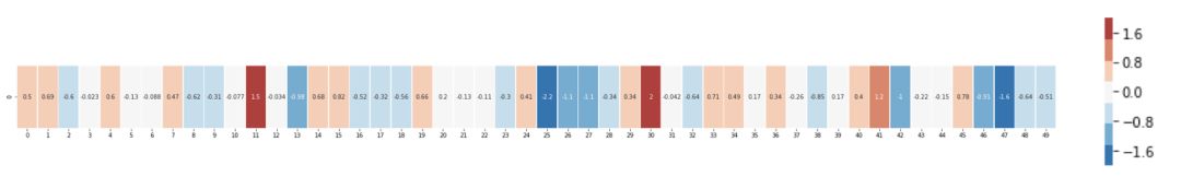
This is the word embedding for the word “king” (trained GloVe vectors on Wikipedia):
[ 0.50451 , 0.68607 , -0.59517 , -0.022801, 0.60046 , -0.13498 , -0.08813 , 0.47377 , -0.61798 , -0.31012 , -0.076666, 1.493 , -0.034189, -0.98173 , 0.68229 , 0.81722 , -0.51874 , -0.31503 , -0.55809 , 0.66421 , 0.1961 , -0.13495 , -0.11476 , -0.30344 , 0.41177 , -2.223 , -1.0756 , -1.0783 , -0.34354 , 0.33505 , 1.9927 , -0.04234 , -0.64319 , 0.71125 , 0.49159 , 0.16754 , 0.34344 , -0.25663 , -0.8523 , 0.1661 , 0.40102 , 1.1685 , -1.0137 , -0.21585 , -0.15155 , 0.78321 , -0.91241 , -1.6106 , -0.64426 , -0.51042 ]
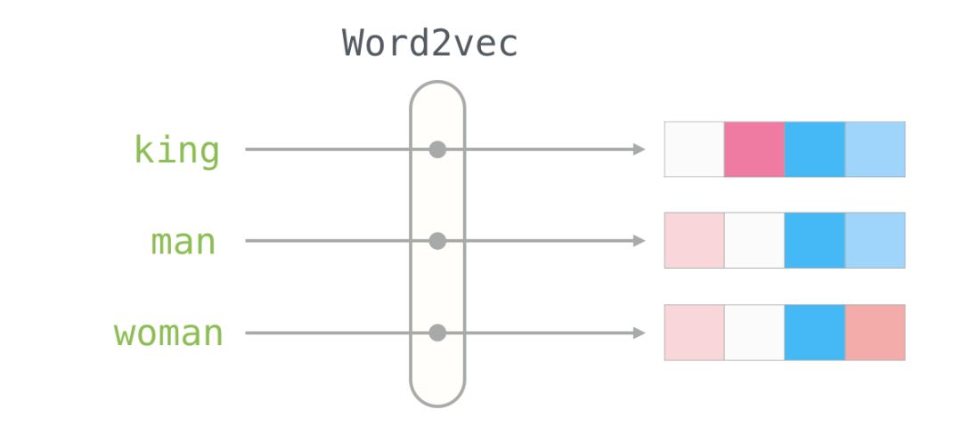
This is a list of 50 numbers. By observing the values, we can’t see much, but let’s visualize it a bit to compare with other word vectors. We put all these numbers in a line:

Let’s color-code the cells based on their values (red for values close to 2, white for values close to 0, and blue for values close to -2):
We will ignore the numbers and only look at the colors to indicate the values of the cells. Now let’s compare “king” with other words:
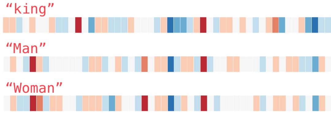
Notice how “man” and “woman” are more similar to each other than either of them is to “king”? This suggests something. These vector visualizations beautifully showcase the information/meaning/association of these words.
This is another example list (look for columns with similar colors by scanning vertically):
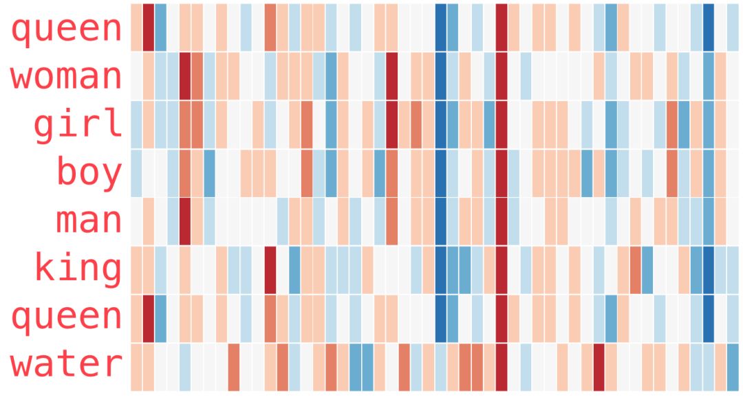
Several points need to be noted:
1. All these different words have a straight red column. They are similar in this dimension (even though we don’t know what each dimension is).
2. You can see that “woman” and “girl” are similar in many respects, and “man” and “boy” are similar as well.
3. “boy” and “girl” also have similarities to each other, but these are different from those with “woman” or “man.” Can these similarities be summarized as a vague concept of “youth”? Perhaps.
4. Except for the last word, all words represent people. I added the object “water” to show the distinctions between categories. You can see that the blue column goes down and stops before the word embedding of “water.”
5. “king” and “queen” are similar to each other, but they differ from other words. Can these be summarized as a vague concept of “royalty”? Perhaps.
Analogy
A famous example showcasing the wonderful properties of embeddings is analogy. We can add and subtract word embeddings to get interesting results. A well-known example is the formula: “king” – “man” + “woman”:
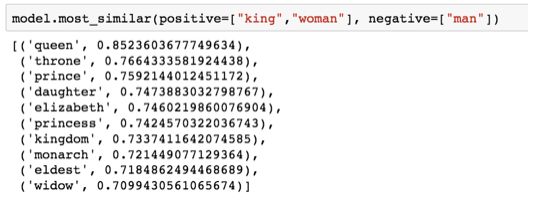
Using the Gensim library in Python, we can add and subtract word vectors, and it will find the words most similar to the resulting vector. This image shows the list of most similar words, each with cosine similarity.
We can visualize this analogy as before:
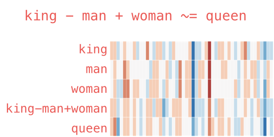
The vector generated by “king – man + woman” is not exactly equal to “queen,” but “queen” is the closest word to it among the 400,000 word embeddings included in this set.
Now that we have seen trained word embeddings, let’s learn more about the training process. But before we start using Word2Vec, we need to look at the parent concept of word embeddings: neural language models.
Language Models
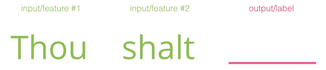
If we were to cite the most typical example of natural language processing, it would probably be the next-word prediction feature in smartphone input methods. This is a feature used hundreds of times every day by billions of people.
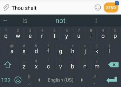
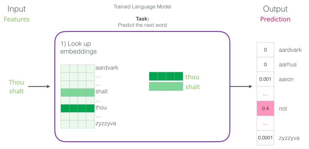
Next-word prediction is a task that can be accomplished by a language model. A language model tries to predict the next word based on a list of words (say, two words).
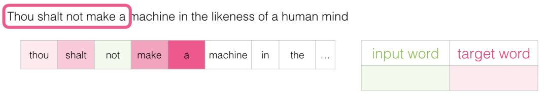
In the above screenshot of a phone, we can consider that the model received two green words (thou shalt) and recommended a set of words (“not” is one of the most likely to be chosen):
We can imagine this model as a black box:
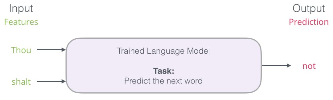
But in fact, the model does not just output one word. In reality, it scores all the words it knows (the model’s vocabulary, which may contain thousands to millions of words) by probability, and the input method program selects the one with the highest score to recommend to the user.
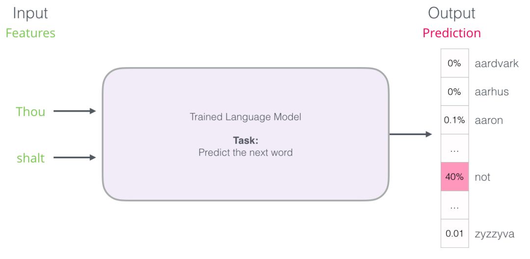
The output of a natural language model is the probability scores of the words known to the model, which we usually express as percentages, but in reality, a score of 40% is represented as 0.4 in the output vector set.
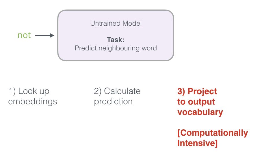
Natural language models (see Bengio 2003) complete predictions in three steps after training, as shown below:
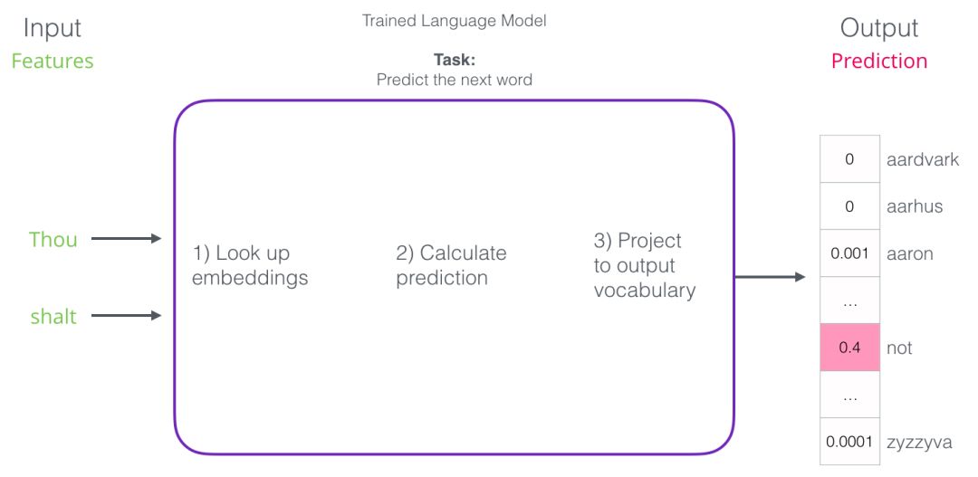
The first step is the most relevant to us because we are discussing Embedding. After training, the model generates a mapping matrix for all words in its vocabulary. During prediction, our algorithm queries the input word in this mapping matrix and calculates the predicted value:
Now let’s focus on model training to learn how to construct this mapping matrix.
Language Model Training
Compared to most other machine learning models, language models have a significant advantage: we have rich text to train language models. All our books, articles, Wikipedia, and various types of text content are available. In contrast, many other machine learning model developments require manually designed data or specially collected data.
We can obtain their mapping relationships by finding words that frequently appear near each other. The mechanism is as follows:
1. First, obtain a large amount of text data (for example, all Wikipedia content)
2. Then we establish a sliding window that can move along the text (for example, a window containing three words)
3. Using this sliding window, we can generate a large sample dataset for training the model.
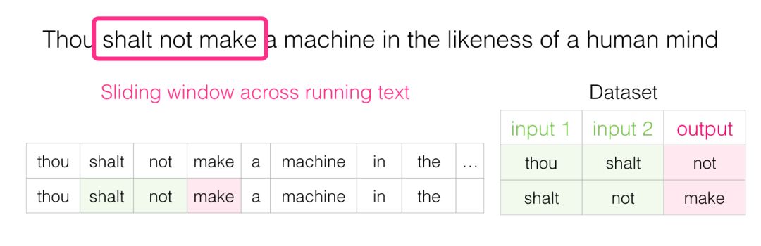
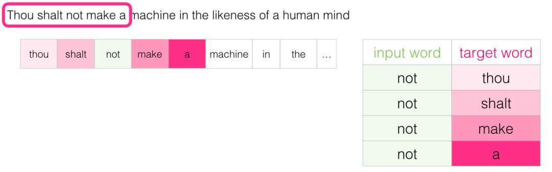
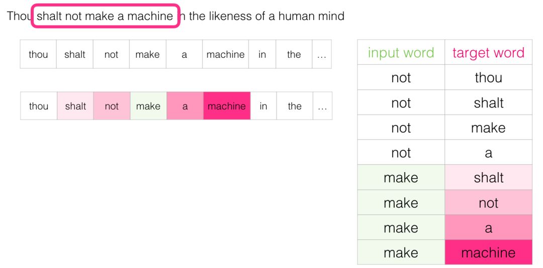
As this window moves along the text, we can (realistically) generate a set of data for model training. To clarify this process, let’s see how the sliding window handles this phrase:
At the beginning, the window locks onto the first three words of the sentence:
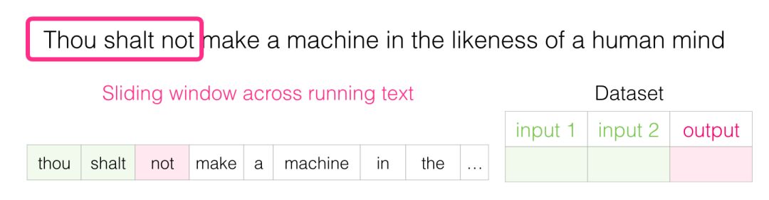
We take the first two words as features and the third word as the label:
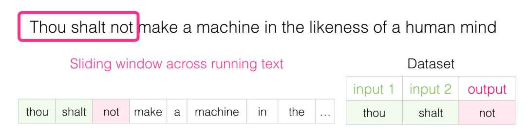
At this point, we have produced the first sample in the dataset, which will be used in our subsequent language model training.
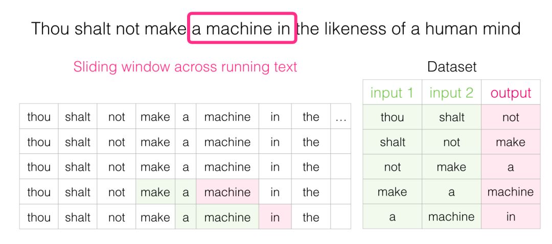
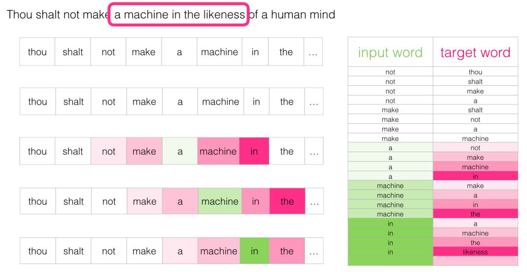
Next, we slide the window to the next position and produce the second sample:
At this point, the second sample has also been generated.
Before long, we can obtain a large dataset, from which we can see the words that appear after different word groups:
In practical applications, the model is often trained as we slide the window. However, I believe separating the generation of the dataset and the training of the model into two stages makes it clearer and easier to understand. Besides using neural networks for modeling, a technique called N-grams is also commonly used for model training.
If you want to understand the transition from using N-grams models to using neural models in real products, you can check out a blog post published by Swiftkey (my favorite Android input method) in 2015, which discusses their natural language model and compares it with earlier N-grams models. I like this example because it tells you how to explain the algorithmic properties of Embedding clearly in marketing presentations.
Consider Both Ends
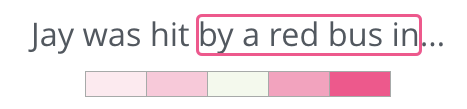
Fill in the blanks based on the previous information:

In front of the blank, the background I provided is five words (if I had mentioned ‘bus’ beforehand), most people would certainly fill in ‘bus’ in the blank. But if I give you another piece of information—like a word after the blank, would the answer change?

Now the content filled in the blank has completely changed. At this time, the word ‘red’ is most likely to fit in that position. From this example, we learn that both the preceding and following words of a word carry informational value. It turns out we need to consider words in both directions (the words on the left and right of the target word). So how can we adjust the training method to accommodate this requirement? Let’s continue to look down.
Skipgram Model
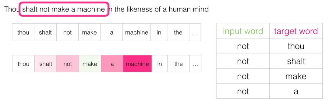
We need to consider not only the two words before the target word but also the two words after it.

If we do this, the model we actually build and train will look like this:
This architecture is called the Continuous Bag of Words (CBOW), as explained in a paper on Word2Vec.
There is another architecture that does not guess the target word based on the context (the preceding and following words) but instead predicts the possible preceding and following words for the current word. Let’s envision how the sliding window looks during training data as illustrated below:
The words in the green box are the input words, and the pink box shows the possible output results.
The depth of the pink box color indicates that the sliding window generates four independent samples for the training set:
This method is called the Skipgram architecture. We can present the contents of the sliding window as shown below.
This provides four samples for the dataset:
Then we move the sliding window to the next position:
This generates the next four samples:
After moving a few positions, we can obtain a batch of samples:
Revisiting the Training Process
Now that we have obtained the training dataset for the Skipgram model from existing text, let’s see how to use it to train a natural language model that predicts adjacent vocabulary.
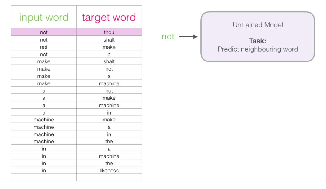
Starting with the first sample in the dataset. We input the features into the untrained model and let it predict a possible adjacent word.
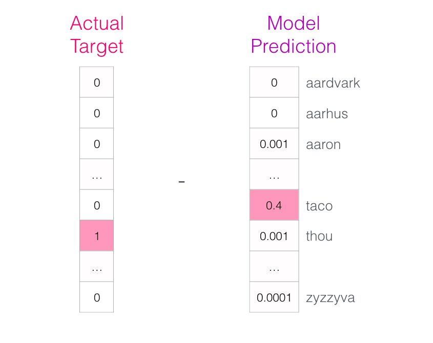
The model will perform three steps and output a prediction vector (corresponding to the probability of each word in the vocabulary). Since the model is untrained, the predictions at this stage are certainly incorrect. But that’s okay; we know which word we should have guessed—that word is the output label in my training data:

The target word probability is 1, while the probabilities of all other words are 0, making the vector composed of these values the “target vector.”
How much bias does the model have? By subtracting the two vectors, we can get the bias vector:
Now this error vector can be used to update the model, so in the next round of predictions, if we use “not” as input, we are more likely to get “thou” as output.

This is actually the first step of training. Next, we continue to perform the same operation on the next sample in the dataset until we have traversed all samples. This constitutes one epoch. We repeat this for several epochs to obtain a trained model, from which we can extract the embedding matrix for other applications.
This certainly helps us understand the entire process, but this is still not the actual training method of Word2Vec. We have missed some key ideas.
Negative Sampling
Recall the three steps the neural language model takes to compute prediction values:
From a computational perspective, the third step is very expensive—especially when we need to do it for each training sample in the dataset (which can easily reach tens of millions). We need to find some ways to improve performance.
One way is to split the target into two steps:
1. Generate high-quality word embeddings (don’t worry about predicting the next word).
2. Use these high-quality embeddings to train the language model (perform next-word prediction).
In this article, we will focus on the first step (because this article focuses on embeddings). To generate high-quality embeddings using high-performance models, we can change the task of predicting adjacent words:
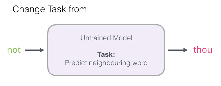
Switch it to a model that extracts input and output words and outputs a score indicating whether they are neighbors (0 means “not neighbors,” 1 means “neighbors”).

This simple transformation changes our required model from a neural network to a logistic regression model—thus it becomes simpler and faster to compute.
This switch requires us to change the structure of the dataset—the label value now has a new column with a value of 0 or 1. They will all be 1 because all the words we added are neighbors.
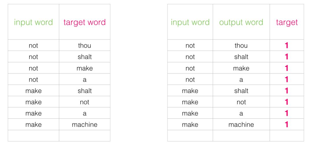
Now the computation speed is incredibly fast—it can process millions of examples in just a few minutes. But we still need to address a loophole. If all examples are neighbors (target: 1), our “genius model” might be trained to always return 1—accuracy is 100%, but it learns nothing and only produces garbage embedding results.
To resolve this issue, we need to introduce negative samples into the dataset—samples of words that are not neighbors. Our model needs to return 0 for these samples. The model must work hard to solve this challenge—and still maintain high speed.
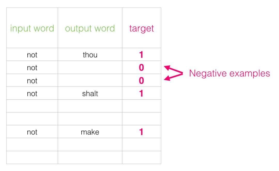
For each sample in our dataset, we add negative examples. They have the same input words, but the labels are 0.
But what do we fill in as output words? We randomly select words from the vocabulary.
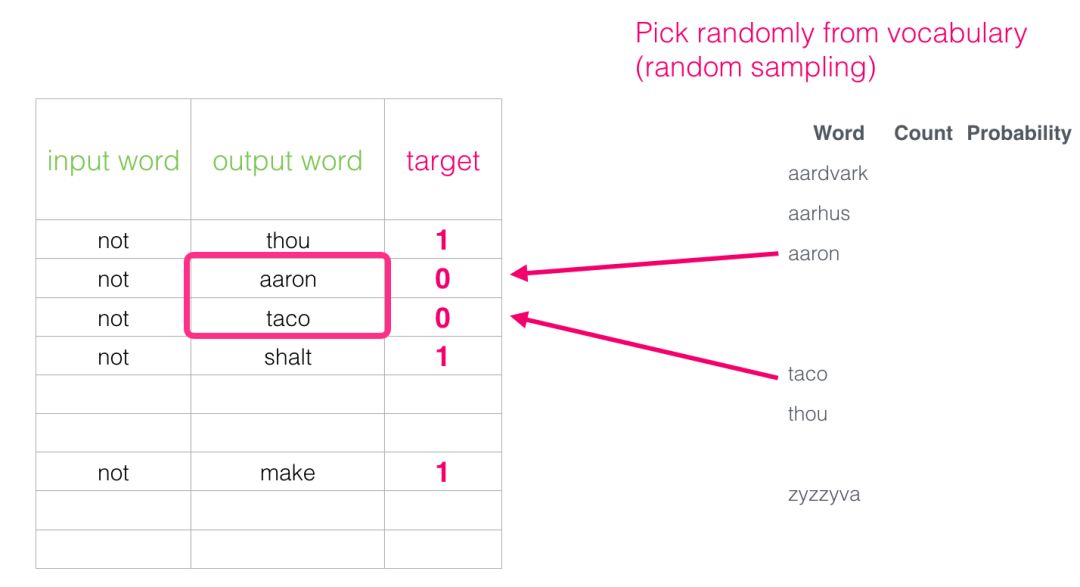
This idea is inspired by noise-contrastive estimation. We compare the actual signal (positive examples of adjacent words) with noise (randomly chosen words that are not neighbors). This leads to a significant trade-off in computational and statistical efficiency.
Noise Contrastive Estimation
http://proceedings.mlr.press/v9/gutmann10a/gutmann10a.pdf
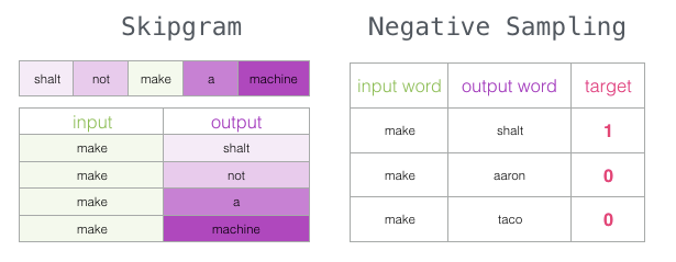
Skipgram with Negative Sampling (SGNS)
We have now introduced two (pairs of) core ideas in Word2Vec: negative sampling and skipgram.
Word2Vec Training Process
Now that we have understood the two core ideas of skipgram and negative sampling, we can continue to closely examine the actual training process of Word2Vec.
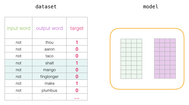
Before the training process begins, we preprocess the text that we are going to train the model on. At this step, we determine the size of the vocabulary (which we call vocab_size, say 10,000) and which words are included in it.
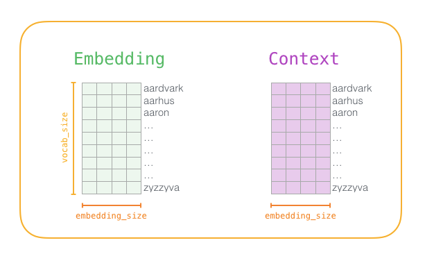
At the beginning of the training phase, we create two matrices—the Embedding matrix and the Context matrix. These two matrices embed each word in our vocabulary (so vocab_size is one of their dimensions). The second dimension is the length we want for each embedding (embedding_size—300 is a common value, but we have also seen examples of 50).
At the start of the training process, we initialize these matrices with random values. Then we begin the training process. In each training step, we take an adjacent example and its related non-adjacent examples. Let’s look at our first set:
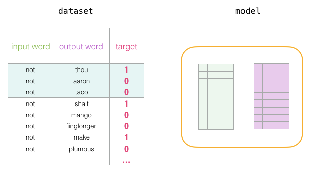
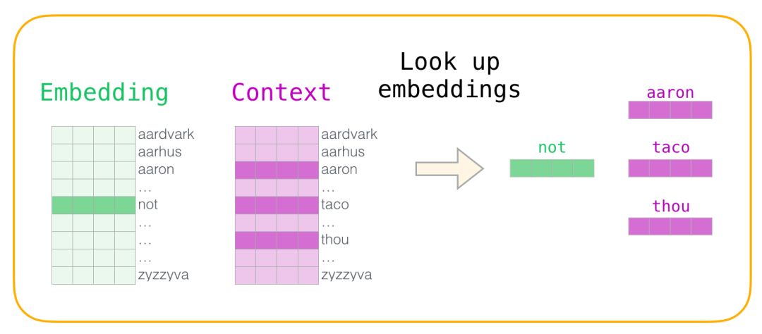
Now we have four words: the input word “not” and the output/context words: “thou” (the actual neighbor word), “aaron,” and “taco” (negative examples). We proceed to look up their embeddings—for the input word, we check the Embedding matrix. For the context words, we check the Context matrix (even though both matrices embed each word in our vocabulary).
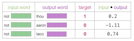
Next, we calculate the dot product of the input embedding with each context embedding. In each case, the result will be a number representing the similarity between the input and context embeddings.
Now we need a way to convert these scores into something that looks like probabilities—we need them to be positive and between 0 and 1. The sigmoid logistic function is perfectly suited for such tasks.
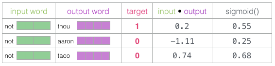
Now we can treat the output of the sigmoid operation as the model output for these examples. You can see that “taco” scores the highest, while “aaron” scores the lowest, both before and after the sigmoid operation.
Since the untrained model has made predictions, and we do have real target labels for comparison, let’s calculate the error in the model’s predictions. To do this, we simply subtract the target labels from the sigmoid scores.
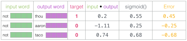
error = target – sigmoid_scores
This is the “learning” part of “machine learning.” Now we can use this error score to adjust the embeddings of “not,” “thou,” “aaron,” and “taco,” so that next time we do this calculation, the results will be closer to the target scores.
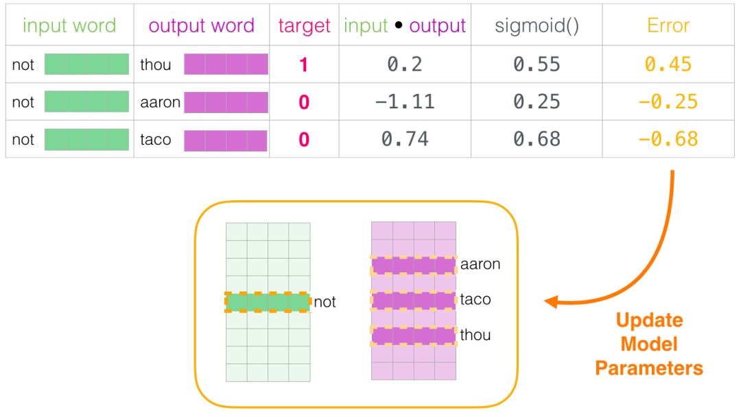
The training step ends here. We have obtained better embeddings for the words used in this step (not, thou, aaron, and taco). We now proceed to the next step (the next adjacent sample and its related non-adjacent samples) and perform the same process again.
As we loop through the dataset multiple times, the embeddings continue to improve. Then we can stop the training process, discard the Context matrix, and use the Embeddings matrix as the trained embeddings for the next task.
Window Size and Number of Negative Samples
Two key hyperparameters in the training process of Word2Vec are the window size and the number of negative samples.
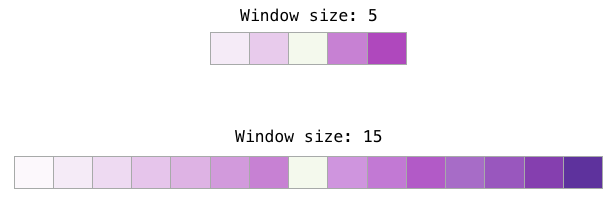
Different tasks suit different window sizes. One heuristic is that using a smaller window size (2-15) will yield embeddings where high similarity scores between two embeddings indicate that these words are interchangeable (note that if we only look at words that are very close, antonyms often can be interchangeable—for example, good and bad often appear in similar contexts). Using a larger window size (15-50 or even more) will yield embeddings where similarity is more indicative of word relevance. In practice, you often need to guide the embedding process to help readers get a similar “sense of language.” Gensim defaults to a window size of 5 (including two words before and after the input word, excluding the input word itself).
 The number of negative samples is another factor affecting the training process. The original paper suggested that 5-20 negative samples is an ideal quantity. It also noted that when you have a sufficiently large dataset, 2-5 seem to be enough. Gensim defaults to 5 negative samples.
Recommended Reading
30 Common Python Functions Carefully Curated
10 Time-Saving PyCharm Tips to Boost Your Productivity!
Give Away 10 Books | Free Shipping | What Are You Waiting For?