Understanding Word2Vec: A Comprehensive Guide

Translation | Yu Zhipeng Lin Xiao Proofreading | Cheng Sijie

Compiled | Kong Lingshuang | AI Study Group

Introduction

The Word2Vec model is used to learn vector representations of words, which we call “word embeddings”. Typically, it serves as a preprocessing step, after which the word vectors are fed into a discriminative model (usually RNN) to generate predictions and perform various interesting operations.

Why Learn Word2Vec

Rich, high-dimensional datasets required for image and sound processing systems are encoded as vectors based on the pixel intensity of each original image, where all information is encoded in such data, allowing for the establishment of various relationships between entities in the system (such as cat and dog).

However, traditional natural language processing systems often treat words as discrete atomic symbols, so cat can be represented as Id537, and dog can be represented as Id143. These encodings are arbitrary and do not provide the system with any information about the relationships between various atomic symbols. This means that when the model processes data about dogs, it cannot relate to the features of cats that the model has already learned (such as they are both animals, both have four legs, both are pets, etc.).

Representing words as unique, discrete IDs also leads to data sparsity and means we may need more data to successfully train statistical models. Using vector representations can avoid these issues.

Let’s Look at an Example

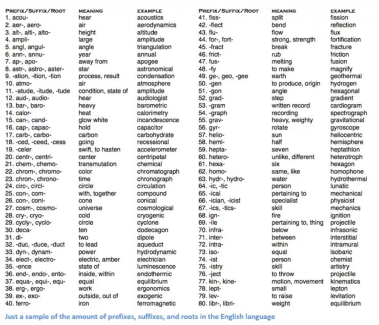
Traditional NLP methods involve a lot of linguistic knowledge, requiring you to understand terms like “phoneme” and “morpheme” because there are many classifications in linguistics, phonetics and morphology being two of them. Let’s see how traditional NLP methods try to understand the following word.

Suppose we want to obtain some information about a word (such as its expressed emotion, its definition, etc.), using linguistic methods we divide the word into three parts: prefix, suffix, and stem.

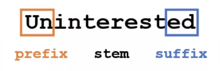
For example, we know that the prefix “un” indicates a negation or opposite meaning, and we also know that “ed” can specify the tense of the word (past tense). We can easily infer the entire meaning and emotion expressed by the word from the stem “interest”. Isn’t it very simple? However, when considering all the different prefixes and suffixes, it requires a very skilled linguist to understand all possible combinations of meanings.

Deep learning is essentially representation learning. We will adopt some methods to create representations of words through training on large datasets.

Word Vectors

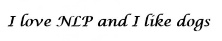
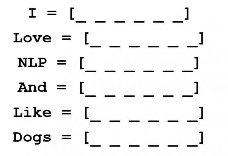
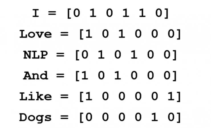
Suppose we represent each word with a d-dimensional vector, where d=6. We want to create word vectors for each unique word in a sentence.

Now consider how to assign values; we want to represent the word and its context, meaning, and semantics in some way. One method is to create a co-occurrence matrix.

A co-occurrence matrix is a matrix that contains the counts of how often this word appears in combination with all other words in the entire corpus (or training set). Let’s take a look at what a co-occurrence matrix looks like.

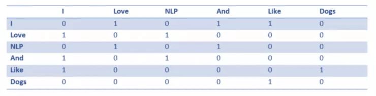
From this simple example of a co-occurrence matrix, we can gather a lot of useful information. For instance, we notice that the word vectors for “love” and “like” both contain several 1s, which count their associated nouns (NLP and dogs). The count for “I” also contains several 1s, indicating that this word must be some verb. When processing large datasets of multiple sentences, you can imagine that this similarity becomes clearer, such as “like”, “love”, and other synonyms will have similar word vectors because they occur in similar contexts.

Currently, although we have a good start, we also need to note that the dimensions of each word will increase linearly with the size of the corpus. If we have one million words (which is not a lot in NLP standards), we will have a one million by one million sized matrix, which is very sparse (with a lot of 0 elements). This is clearly not the best solution in terms of storage efficiency. There have been many improvements in finding the best way to represent these word vectors. The most famous of these is Word2Vec.

Formal Introduction

Vector space models (VSMs) represent (embed) words in a continuous vector space, where semantically similar words are mapped to nearby points (embedded near each other). VSMs have a long history in the development of NLP, but they all rely on the distributional hypothesis, which states that words that appear in the same context have similar semantics. Methods that utilize this principle can be divided into two categories:

1. Count-based methods (e.g., Latent Semantic Analysis);

2. Predictive methods (e.g., neural probabilistic language models)

Their distinction is–

Count-based methods calculate statistics of how often a word co-occurs with its neighboring vocabulary in a large text corpus and then map each word of these statistics to a small and dense vector.

Predictive models directly attempt to predict words from their neighbors based on learned small dense embedding vectors (considering the parameters of the model).

Word2Vec is a particularly effective predictive model for learning word embeddings from raw text. It has two forms, namely Continuous Bag of Words (CBOW) and the Skip-Gram model. Algorithmically, these models are similar, except that CBOW predicts the target word from the source context words, while the Skip-Gram does the opposite and predicts the words from the target word’s source context.

In the next discussion, we will focus on the Skip-Gram model.

Mathematical Application

Traditionally, neural probabilistic language models are trained using the maximum likelihood principle to maximize the probability of the next word wt (“target”) given the previous word h (“history”) in the form of a softmax function.

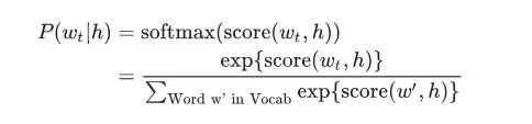
Using score(wt, h) to calculate the compatibility of the target word wt with the context h (usually using dot product operations).

We train this model by maximizing its log likelihood on the training set. So, we maximize the following loss function.

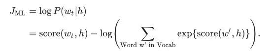
This provides a suitable normalized probability model for language modeling.

This same argument can also be represented with a slightly different formula, which clearly shows the variables (or parameters) that change to maximize this objective.

Our goal is to find some word representations that can be used to predict the surrounding vocabulary of the current word. Specifically, we want to maximize the average log probability of our entire corpus:

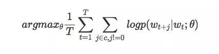
This equation essentially has some probability p of observing the current word wt within a specific word of size c. This probability depends on the current word wt and some settings of parameters θ (determined by our model). We want to set these parameters θ to maximize this probability across the entire corpus.

Basic Parameterization: Softmax Model

The basic Skip-Gram model defines the probability p through the softmax function, as we have seen earlier. If we consider the dimension of wi to be N and θ as a one-hot encoded vector, and it is an N×K matrix embedding matrix, representing that we have N words in our vocabulary and the embeddings we learn have a dimension of K, we can define –

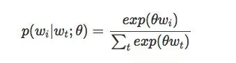
It is worth noting that after learning, the matrix theta can be considered as an embedding lookup matrix.

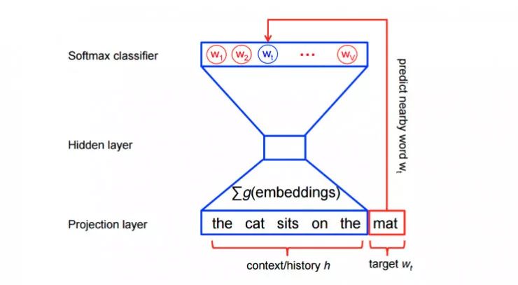
In terms of architecture, it is a simple three-layer neural network.

1. Build a three-layer network structure (one input layer, one hidden layer, one output layer)

2. Input a word and let it train its nearby words

3. Remove the output layer but keep the input and hidden layers

4. Then, input a word from the vocabulary. The output given by the hidden layer is the “word embedding” of the input word

This parameterization has a major drawback, limiting its usefulness in large corpora. Specifically, we note that to compute a single forward pass of our model, we must summarize the entire vocabulary of the corpus to evaluate the softmax function. This is very extravagant for large datasets, so we consider alternative approximations for computational efficiency.

Improving Computational Efficiency

For feature learning in Word2Vec, we do not need a complete probability model. The CBOW and Skip-Gram models are trained using a binary classification objective (logistic regression) to distinguish the real target word (wt) from k negative (noise) words w in the same context.

In mathematical terms, this operation is maximization over each object.

This objective is maximized when the model assigns high probabilities to real words and low probabilities to noise words. Technically, this is known as negative sampling, which proposes updates that approximate the updates of the softmax function in the limit. However, computationally it is particularly attractive because the computation of the loss function now only depends on the number of noise words we choose (k) rather than all words in the vocabulary (V), making it train faster. Packages like TensorFlow use a very similar loss function called Noise Contrastive Estimation (NCE) loss.

Intuition Behind the Skip-Gram Model

As an example, we need to consider the dataset –

the quick brown fox jumped over the lazy dog

We first form a word dataset and their contexts. Now, let’s stick with the vanilla definition and define “context” as the target word’s left and right word window. Using a window size of 1, we have a dataset of (context, target) pairs.

([the, brown], quick), ([quick, fox], brown), ([brown, jumped], fox), …

Recall that Skip-Gram reverses the context and target and tries to predict each context word from the target word, so the task will predict “the” and “brown” from “quick”, “quick”, and “fox”.

Thus our dataset becomes (input, output), as follows:

(quick, the), (quick, brown), (brown, quick), (brown, fox), …

The objective function is defined over the entire dataset, but we typically optimize each example (or a “minibatch” of batch_size examples, typically 16 <= batch_size <= 512) using stochastic gradient descent (SGD). Let’s take a look at one step of this process.

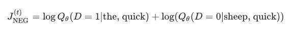
Let’s imagine that during the training step, we observe the first training case above, where the target is to predict quick. We select the number of noise (contrast) examples num_noise from some noise distribution (usually a unigram distribution) (this unit assumes that the occurrence of each word is independent of the occurrences of all other words, meaning we can view the generation process as a sequence of dice rolls P(w).

For simplicity, let’s assume num_noise = 1, and we choose sheep as a noise example. Next, we calculate the loss for this pair of observed and noise examples, i.e., at time step “t” the target becomes –

Our goal is to update the embedding parameters θ to maximize this objective function. We do this by deriving the loss gradient with respect to the embedding parameters θ.

Then, we update the embedding parameters by moving in the direction of the gradient. When this process is repeated over the entire training set, it has the effect of “moving” the embedding vectors for each word until the model successfully distinguishes real words from noise words.

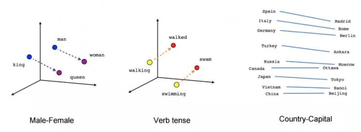
We can visualize the learned vectors by projecting them down to 3 dimensions. When we observe these visualized variables, it is clear that these vectors capture some semantic information about the words and their relationships, which is very useful in practical applications.

References

1. TensorFlow implementation of Word2Vec

   https://www.tensorflow.org/tutorials/word2vec

2. Distributed Representations of Words and Phrases and their Compositionality – Research Paper by Tomas Mikolov, Ilya Sutskever, Kai Chen, Greg Corrado, and Jeffrey Dean

   https://papers.nips.cc/paper/5021-distributed-representations-of-words-and-phrases-and-their-compositionality.pdf

3. A Practical Guide to Word2Vec by Aneesh Joshi

   https://towardsdatascience.com/learn-word2vec-by-implementing-it-in-tensorflow-45641adaf2ac

4. Review of Natural Language by Adit Deshpande

   https://adeshpande3.github.io/adeshpande3.github.io/Deep-Learning-Research-Review-Week-3-Natural-Language-Processing

5. Language Models by Rohan Verma

   http://rohanvarma.me/Word2Vec/