
Source: Deep Learning Enthusiasts


This article is about 8000 words long and is recommended to be read in 16 minutes.
This article will detail the Vision Transformer (ViT) explained in "An Image is Worth 16x16 Words".
Since the concept of “Attention is All You Need” was introduced in 2017, Transformer models have quickly emerged in the field of Natural Language Processing (NLP), establishing their leading position. By 2021, the idea that “An image is worth 16×16 words” successfully brought Transformer models into computer vision tasks. Since then, numerous Transformer-based architectures have emerged and been applied in the field of computer vision.
This article will detail the Vision Transformer (ViT) as explained in “An Image is Worth 16×16 Words”, including its open-source code and conceptual explanations of each component. All code is implemented using the PyTorch Python package.
This article is part of a series that delves into the inner workings of Vision Transformers, providing an executable code version in Jupyter Notebook. Other articles in the series include: Understanding Vision Transformers, Applications of Attention Mechanism in Vision Transformers, Analysis of Positional Encoding in Vision Transformers, Tokens-to-Token Vision Transformers, and the GitHub repository for the Vision Transformers series.
So, what are Vision Transformers? As introduced in “Attention is All You Need”, Transformers are machine learning models that use attention mechanisms as their primary learning mechanism. They quickly became the leading technology for sequence-to-sequence tasks (such as language translation).
“An image is worth 16×16 words” successfully improved the Transformer proposed in [1] to handle image classification tasks, giving rise to Vision Transformer (ViT). Similar to the Transformer used for NLP tasks, ViT is based on attention mechanisms. However, unlike the Transformer for NLP tasks which contains both encoder and decoder attention branches, ViT uses only the encoder. The output of the encoder is then passed to the neural network head for prediction.
However, the ViT implemented in “An Image is Worth 16×16 Words” has a drawback: its optimal performance requires pre-training on large datasets. The best model was pre-trained on the proprietary JFT-300M dataset. Meanwhile, models pre-trained on the smaller open-source ImageNet-21k dataset perform comparably to state-of-the-art convolutional ResNet models.
Tokens-to-Token ViT: Training Vision Transformers from Scratch on ImageNet attempts to eliminate this pre-training requirement by introducing a novel preprocessing method that converts input images into a series of tokens. For more information about this method, please refer to the relevant materials. In this article, we will focus on the ViT implemented in “An Image is Worth 16×16 Words”.
Model Analysis
This article follows the model structure outlined in “An Image is Worth 16×16 Words”. However, the code from that paper has not been publicly released. The code from the recent “Tokens-to-Token ViT” can be found on GitHub. The Tokens-to-Token ViT (T2T-ViT) model adds a Tokens-to-Token (T2T) module before the standard ViT backbone structure. The code in this article is based on the ViT components from the “Tokens-to-Token ViT” GitHub code. The code has been modified to allow for non-square input images and removed the dropout layers.
A schematic diagram of the ViT model structure is shown below.
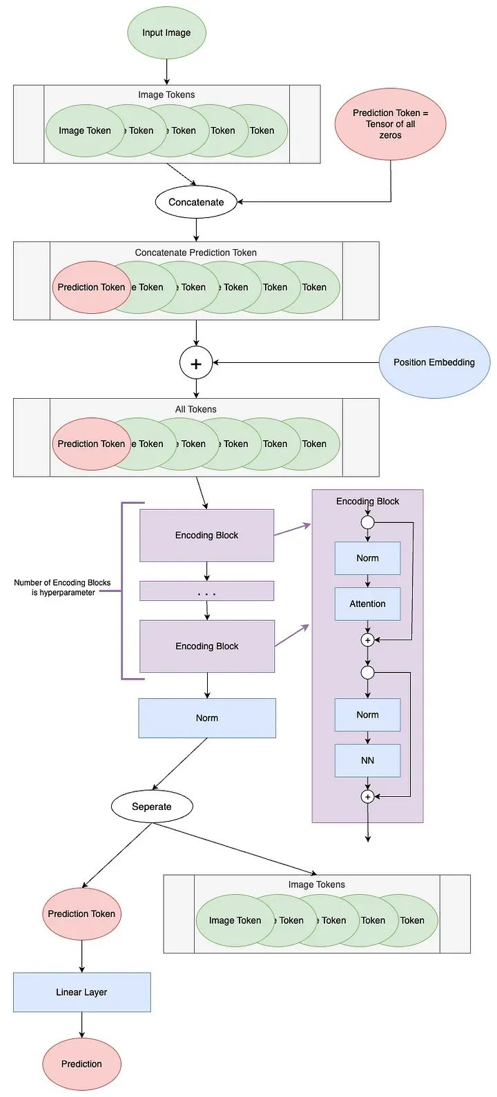
Image Tokenization
The first step of ViT is to create tokens from the input image. Transformers operate on a series of tokens; in NLP, this is usually the words of a sentence. For computer vision, how to segment the input into tokens is not very clear.
ViT converts an image into tokens such that each token represents a local area (or patch) of the image. They describe how to reshape an image with height H, width W, and channel count C into N patches of size P:
Each token has a length of P²*C.
Let’s take this pixel art “Mountain at Dusk” (by Luis Zuno) as an example for patch tokenization. The original artwork has been cropped and converted to a single-channel image. This means that the value of each pixel is between 0 and 1. Single-channel images are usually displayed in grayscale, but we will display it with a purple color scheme for better visibility. Note that the patch tokenization is not included in the relevant code in [3].
mountains = np.load(os.path.join(figure_path, 'mountains.npy'))
H = mountains.shape[0]
W = mountains.shape[1]
print('Mountain at Dusk is H =', H, 'and W =', W, 'pixels.')
print('\n')
fig = plt.figure(figsize=(10,6))
plt.imshow(mountains, cmap='Purples_r')
plt.xticks(np.arange(-0.5, W+1, 10), labels=np.arange(0, W+1, 10))
plt.yticks(np.arange(-0.5, H+1, 10), labels=np.arange(0, H+1, 10))
plt.clim([0,1])
cbar_ax = fig.add_axes([0.95, .11, 0.05, 0.77])
plt.clim([0, 1])
plt.colorbar(cax=cbar_ax);
#plt.savefig(os.path.join(figure_path, 'mountains.png'))
Mountain at Dusk is H = 60 and W = 100 pixels.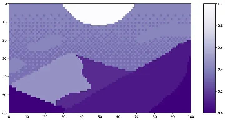
The height of this image is H=60, and the width is W=100. We will set P=20, as it can evenly divide H and W.
P = 20
N = int((H*W)/(P**2))
print('There will be', N, 'patches, each', P, 'by', str(P)+'.')
print('\n')
fig = plt.figure(figsize=(10,6))
plt.imshow(mountains, cmap='Purples_r')
plt.hlines(np.arange(P, H, P)-0.5, -0.5, W-0.5, color='w')
plt.vlines(np.arange(P, W, P)-0.5, -0.5, H-0.5, color='w')
plt.xticks(np.arange(-0.5, W+1, 10), labels=np.arange(0, W+1, 10))
plt.yticks(np.arange(-0.5, H+1, 10), labels=np.arange(0, H+1, 10))
x_text = np.tile(np.arange(9.5, W, P), 3)
y_text = np.repeat(np.arange(9.5, H, P), 5)
for i in range(1, N+1):    plt.text(x_text[i-1], y_text[i-1], str(i), color='w', fontsize='xx-large', ha='center')
plt.text(x_text[2], y_text[2], str(3), color='k', fontsize='xx-large', ha='center');
#plt.savefig(os.path.join(figure_path, 'mountain_patches.png'), bbox_inches='tight')
There will be 15 patches, each 20 by 20.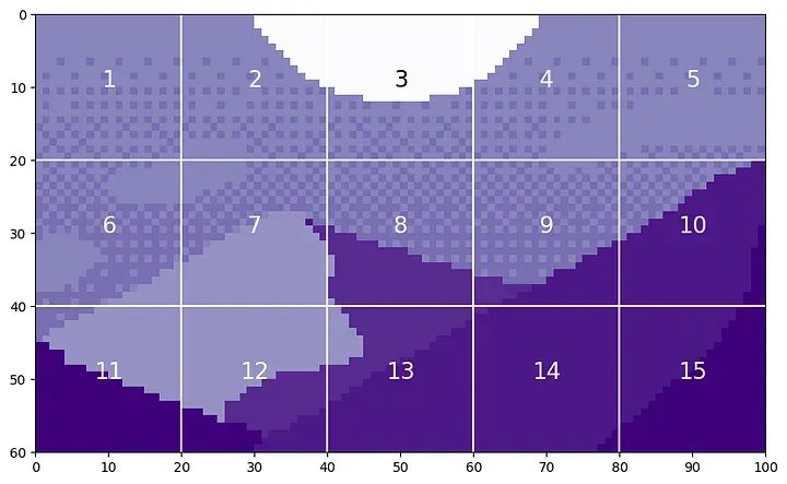
By flattening these patches, we can see the generated tokens. Let’s take the 12th patch as an example, as it contains four different tones.
print('Each patch will make a token of length', str(P**2)+'.')
print('\n')
patch12 = mountains[40:60, 20:40]
token12 = patch12.reshape(1, P**2)
fig = plt.figure(figsize=(10,1))
plt.imshow(token12, aspect=10, cmap='Purples_r')
plt.clim([0,1])
plt.xticks(np.arange(-0.5, 401, 50), labels=np.arange(0, 401, 50))
plt.yticks([]);
#plt.savefig(os.path.join(figure_path, 'mountain_token12.png'), bbox_inches='tight')
Each patch will make a token of length 400.
After extracting tokens from the image, linear projection is usually applied to change the length of the tokens. This is achieved through a learnable linear layer. The new token length is referred to as the latent dimension, channel dimension, or token length. After the projection, the tokens can no longer be visually identified as patches of the original image. Now that we understand this concept, let’s see how patch tokenization is implemented in code.
class Patch_Tokenization(nn.Module):    def __init__(self,                img_size: tuple[int, int, int]=(1, 1, 60, 100),                patch_size: int=50,                token_len: int=768):
        """ Patch Tokenization Module            Args:                img_size (tuple[int, int, int]): size of input (channels, height, width)                patch_size (int): the side length of a square patch                token_len (int): desired length of an output token        """        super().__init__()
        ## Defining Parameters        self.img_size = img_size        C, H, W = self.img_size        self.patch_size = patch_size        self.token_len = token_len        assert H % self.patch_size == 0, 'Height of image must be evenly divisible by patch size.'        assert W % self.patch_size == 0, 'Width of image must be evenly divisible by patch size.'        self.num_tokens = (H / self.patch_size) * (W / self.patch_size)
        ## Defining Layers        self.split = nn.Unfold(kernel_size=self.patch_size, stride=self.patch_size, padding=0)        self.project = nn.Linear((self.patch_size**2)*C, token_len)
    def forward(self, x):        x = self.split(x).transpose(1,0)        x = self.project(x)        return x
Note the two assert statements, which ensure that the image dimensions can be evenly divided by the patch size. The actual patch division is implemented through a torch.nn.Unfold⁵ layer.
We will use our cropped single-channel version of Mountain at Dusk⁴ to run an example of this code. We should see the same number of tokens and initial token size as before. The first line of the code block below changes the data type of Mountain at Dusk⁴ from a NumPy array to a Torch tensor. We also need to perform an unsqueeze⁶ operation on the tensor to create a channel dimension and a batch size dimension. Like above, we only have one channel. Since there is only one image, the batch size is 1.
x = torch.from_numpy(mountains).unsqueeze(0).unsqueeze(0).to(torch.float32)
token_len = 768
print('Input dimensions are\n\tbatchsize:', x.shape[0], '\n\tnumber of input channels:', x.shape[1], '\n\timage size:', (x.shape[2], x.shape[3]))
# Define the Module
patch_tokens = Patch_Tokenization(img_size=(x.shape[1], x.shape[2], x.shape[3]),                                    patch_size = P,                                    token_len = token_len)
Input dimensions are batchsize: 1 number of input channels: 1 image size: (60, 100)As we saw in the example, there are a total of N=15 tokens with a length of 400. Finally, we will project the tokens to token_len.
x = patch_tokens.split(x).transpose(2,1)
print('After patch tokenization, dimensions are\n\tbatchsize:', x.shape[0], '\n\tnumber of tokens:', x.shape[1], '\n\ttoken length:', x.shape[2])
After patch tokenization, dimensions are batchsize: 1 number of tokens: 15 token length: 400Now that we have the tokens, we are ready to proceed with ViT.
Token Processing
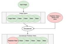
We will refer to the next two steps of ViT, prior to the encoding blocks, as “Token Processing”. The components of token processing in the ViT diagram are shown below.
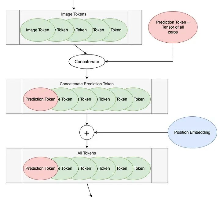
The first step is to add a blank token before the image tokens, called the Prediction Token. This token will be used to output the encoding blocks for prediction. It starts off blank – equivalent to zero – so it can gather information from other image tokens.
# Define an Input
num_tokens = 175
token_len = 768
batch = 13
x = torch.rand(batch, num_tokens, token_len)
print('Input dimensions are\n\tbatchsize:', x.shape[0], '\n\tnumber of tokens:', x.shape[1], '\n\ttoken length:', x.shape[2])
# Append a Prediction Token
pred_token = torch.zeros(1, 1, token_len).expand(batch, -1, -1)
print('Prediction Token dimensions are\n\tbatchsize:', pred_token.shape[0], '\n\tnumber of tokens:', pred_token.shape[1], '\n\ttoken length:', pred_token.shape[2])
x = torch.cat((pred_token, x), dim=1)
print('Dimensions with Prediction Token are\n\tbatchsize:', x.shape[0], '\n\tnumber of tokens:', x.shape[1], '\n\ttoken length:', x.shape[2])
Input dimensions are batchsize: 13 number of tokens: 175 token length: 768
Prediction Token dimensions are batchsize: 13 number of tokens: 1 token length: 768
Dimensions with Prediction Token are batchsize: 13 number of tokens: 176 token length: 768We will start with 175 tokens. Each token has a length of 768, which is the size of the ViT² base variant. We use a batch size of 13 as it is prime and will not confuse with other parameters.
def get_sinusoid_encoding(num_tokens, token_len):    """ Make Sinusoid Encoding Table
        Args:            num_tokens (int): number of tokens            token_len (int): length of a token
        Returns:            (torch.FloatTensor) sinusoidal position encoding table    """
    def get_position_angle_vec(i):        return [i / np.power(10000, 2 * (j // 2) / token_len) for j in range(token_len)]
    sinusoid_table = np.array([get_position_angle_vec(i) for i in range(num_tokens)])    sinusoid_table[:, 0::2] = np.sin(sinusoid_table[:, 0::2])    sinusoid_table[:, 1::2] = np.cos(sinusoid_table[:, 1::2])
    return torch.FloatTensor(sinusoid_table).unsqueeze(0)
PE = get_sinusoid_encoding(num_tokens+1, token_len)
print('Position embedding dimensions are\n\tnumber of tokens:', PE.shape[1], '\n\ttoken length:', PE.shape[2])
x = x + PE
print('Dimensions with Position Embedding are\n\tbatchsize:', x.shape[0], '\n\tnumber of tokens:', x.shape[1], '\n\ttoken length:', x.shape[2])
Position embedding dimensions are number of tokens: 176 token length: 768
Dimensions with Position Embedding are batchsize: 13 number of tokens: 176 token length: 768Now, we have added a positional embedding to our tokens. Positional embeddings allow the Transformer to understand the order of the image tokens. Note that this is an addition, not a concatenation. The specifics of positional embeddings are a topic worth discussing later.
def get_sinusoid_encoding(num_tokens, token_len):    """ Make Sinusoid Encoding Table
        Args:            num_tokens (int): number of tokens            token_len (int): length of a token
        Returns:            (torch.FloatTensor) sinusoidal position encoding table    """
    def get_position_angle_vec(i):        return [i / np.power(10000, 2 * (j // 2) / token_len) for j in range(token_len)]
    sinusoid_table = np.array([get_position_angle_vec(i) for i in range(num_tokens)])    sinusoid_table[:, 0::2] = np.sin(sinusoid_table[:, 0::2])    sinusoid_table[:, 1::2] = np.cos(sinusoid_table[:, 1::2])
    return torch.FloatTensor(sinusoid_table).unsqueeze(0)
PE = get_sinusoid_encoding(num_tokens+1, token_len)
print('Position embedding dimensions are\n\tnumber of tokens:', PE.shape[1], '\n\ttoken length:', PE.shape[2])
x = x + PE
print('Dimensions with Position Embedding are\n\tbatchsize:', x.shape[0], '\n\tnumber of tokens:', x.shape[1], '\n\ttoken length:', x.shape[2])
Position embedding dimensions are number of tokens: 176 token length: 768
Dimensions with Position Embedding are batchsize: 13 number of tokens: 176 token length: 768Now our tokens are ready to enter the encoding blocks.
Encoding Blocks
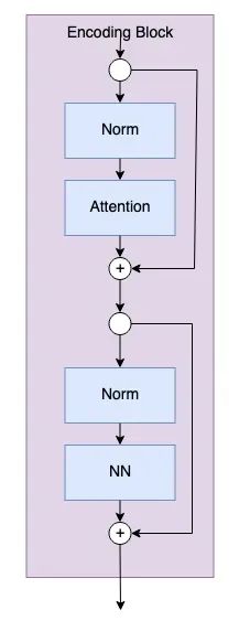
Encoding blocks are where the model actually learns from the image tokens. The number of encoding blocks is a hyperparameter set by the user. The diagram of encoding blocks is shown below.
The code for the encoding blocks is as follows.
class Encoding(nn.Module): def __init__(self, dim: int, num_heads: int=1, hidden_chan_mul: float=4., qkv_bias: bool=False, qk_scale: NoneFloat=None, act_layer=nn.GELU, norm_layer=nn.LayerNorm): """ Encoding Block Args: dim (int): size of a single token num_heads(int): number of attention heads in MSA hidden_chan_mul (float): multiplier to determine the number of hidden channels (features) in the NeuralNet component qkv_bias (bool): determines if the qkv layer learns an additive bias qk_scale (NoneFloat): value to scale the queries and keys by; if None, queries and keys are scaled by ``head_dim ** -0.5`` act_layer(nn.modules.activation): torch neural network layer class to use as activation norm_layer(nn.modules.normalization): torch neural network layer class to use as normalization """ super().__init__() ## Define Layers self.norm1 = norm_layer(dim) self.attn = Attention(dim=dim, chan=dim, num_heads=num_heads, qkv_bias=qkv_bias, qk_scale=qk_scale) self.norm2 = norm_layer(dim) self.neuralnet = NeuralNet(in_chan=dim, hidden_chan=int(dim*hidden_chan_mul), out_chan=dim, act_layer=act_layer) def forward(self, x): x = x + self.attn(self.norm1(x)) x = x + self.neuralnet(self.norm2(x)) return xThe parameters num_heads, qkv_bias, and qk_scale define the components of the attention module. An in-depth study of the attention in vision transformers will be discussed next time.
The parameters hidden_chan_mul and act_layer define the neural network module components. The activation layer can be any layer⁷. We will detail the neural network module later on.
Any layer can be chosen for the norm_layer torch.nn.modules.normalization.
Now, we will go through each blue block in the diagram step by step along with the accompanying code. We will use 176 tokens with a length of 768. We will use a batch size of 13 as it is prime and will not confuse with other parameters. We will use 4 attention heads as it divides evenly into the token length; however, you will not see the attention head dimension in the encoding block.
# Define an Input
num_tokens = 176
token_len = 768
batch = 13
heads = 4
x = torch.rand(batch, num_tokens, token_len)
print('Input dimensions are\n\tbatchsize:', x.shape[0], '\n\tnumber of tokens:', x.shape[1], '\n\ttoken length:', x.shape[2])
# Define the Module
E = Encoding(dim=token_len, num_heads=heads, hidden_chan_mul=1.5, qkv_bias=False, qk_scale=None, act_layer=nn.GELU, norm_layer=nn.LayerNorm)
E.eval();
Input dimensions are batchsize: 13 number of tokens: 176 token length: 768Now we will pass through a norm layer and an attention module. The attention module in the encoding block is parameterized, so it does not change the token length. After the attention module, we implement the first split connection.
y = E.norm1(x)
print('After norm, dimensions are\n\tbatchsize:', y.shape[0], '\n\tnumber of tokens:', y.shape[1], '\n\ttoken size:', y.shape[2])
y = E.attn(y)
print('After attention, dimensions are\n\tbatchsize:', y.shape[0], '\n\tnumber of tokens:', y.shape[1], '\n\ttoken size:', y.shape[2])
y = y + x
print('After split connection, dimensions are\n\tbatchsize:', y.shape[0], '\n\tnumber of tokens:', y.shape[1], '\n\ttoken size:', y.shape[2])
After norm, dimensions are batchsize: 13 number of tokens: 176 token size: 768
After attention, dimensions are batchsize: 13 number of tokens: 176 token size: 768
After split connection, dimensions are batchsize: 13 number of tokens: 176 token size: 768Now, we go through another norm layer followed by the neural network module. Finally, we have the second split connection.
z = E.norm2(y)
print('After norm, dimensions are\n\tbatchsize:', z.shape[0], '\n\tnumber of tokens:', z.shape[1], '\n\ttoken size:', z.shape[2])
z = E.neuralnet(z)
print('After neural net, dimensions are\n\tbatchsize:', z.shape[0], '\n\tnumber of tokens:', z.shape[1], '\n\ttoken size:', z.shape[2])
z = z + y
print('After split connection, dimensions are\n\tbatchsize:', z.shape[0], '\n\tnumber of tokens:', z.shape[1], '\n\ttoken size:', z.shape[2])
After norm, dimensions are batchsize: 13 number of tokens: 176 token size: 768
After neural net, dimensions are batchsize: 13 number of tokens: 176 token size: 768
After split connection, dimensions are batchsize: 13 number of tokens: 176 token size: 768This is the entire content of a single encoding block! Since the final dimension is the same as the initial dimension, the model can easily pass tokens through multiple encoding blocks, set by the depth hyperparameter.
Neural Network Module
The Neural Network (NN) module is a subcomponent of the encoding block. The NN module is very simple, consisting of a fully connected layer, an activation layer, and another fully connected layer. The activation layer can be any layer from torch.nn.modules.activation⁷, passed as input to the module. The NN module can be configured to change the shape of the input or keep the same shape. We will not go through this code step by step as neural networks are common in machine learning and are not the focus of this article. However, the code for the NN module is given below.
class NeuralNet(nn.Module):    def __init__(self,       in_chan: int,       hidden_chan: NoneFloat=None,       out_chan: NoneFloat=None,       act_layer = nn.GELU):        """ Neural Network Module
            Args:                in_chan (int): number of channels (features) at input                hidden_chan (NoneFloat): number of channels (features) in the hidden layer;                                        if None, number of channels in hidden layer is the same as the number of input channels                out_chan (NoneFloat): number of channels (features) at output;                                        if None, number of output channels is same as the number of input channels                act_layer(nn.modules.activation): torch neural network layer class to use as activation        """
        super().__init__()
        ## Define Number of Channels        hidden_chan = hidden_chan or in_chan
Prediction Processing
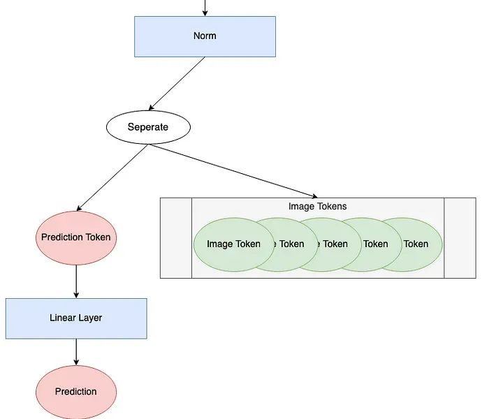
After the encoding blocks, the last thing the model must do is make predictions. The “Prediction Processing” component in the ViT diagram is shown below.
We will look at each step of this process. We will continue to use 176 tokens with a length of 768. We will use a batch size of 1 to illustrate how to make a single prediction. A batch size greater than 1 will compute this prediction in parallel.
# Define an Input
num_tokens = 176
token_len = 768
batch = 1
x = torch.rand(batch, num_tokens, token_len)
print('Input dimensions are\n\tbatchsize:', x.shape[0], '\n\tnumber of tokens:', x.shape[1], '\n\ttoken length:', x.shape[2])
Input dimensions are batchsize: 1 number of tokens: 176 token length: 768First, all tokens go through a norm layer.
norm = nn.LayerNorm(token_len)
x = norm(x)
print('After norm, dimensions are\n\tbatchsize:', x.shape[0], '\n\tnumber of tokens:', x.shape[1], '\n\ttoken size:', x.shape[2])
Next, we separate out the prediction token from the remaining tokens. In the encoding block, the prediction token has become non-zero and has gathered information about our input image. We will use only this prediction token for the final prediction.
norm = nn.LayerNorm(token_len)
pred_token = x[:, 0]
print('Length of prediction token:', pred_token.shape[-1])
Length of prediction token: 768Finally, we pass the prediction token to the head for prediction. The head is usually some type of neural network that varies depending on the model. In “An Image is Worth 16×16 Words²”, they used an MLP (multi-layer perceptron) with one hidden layer during pre-training and a single linear layer during fine-tuning. In “Tokens-to-Token ViT³”, they used a single linear layer as the head. This example will use an output shape of 1 to represent a single estimated regression value.
head = nn.Linear(token_len, 1)
pred = head(pred_token)
print('Length of prediction:', (pred.shape[0], pred.shape[1]))
print('Prediction:', float(pred))
Length of prediction: (1, 1)
Prediction: -0.5474240779876709That’s it! The model has made a prediction!
Complete Code
To create the complete ViT module, we use the Patch Tokenization module and the ViT Backbone module defined above. The ViT Backbone is defined as follows, containing the Token Processing, Encoding Blocks, and Prediction Processing components.
class ViT_Backbone(nn.Module):    def __init__(self,                preds: int=1,                token_len: int=768,                num_heads: int=1,                Encoding_hidden_chan_mul: float=4.,                depth: int=12,                qkv_bias=False,                qk_scale=None,                act_layer=nn.GELU,                norm_layer=nn.LayerNorm):
        """ VisTransformer Backbone            Args:                preds (int): number of predictions to output                token_len (int): length of a token                num_heads(int): number of attention heads in MSA                Encoding_hidden_chan_mul (float): multiplier to determine the number of hidden channels (features) in the NeuralNet component of the Encoding Module                depth (int): number of encoding blocks in the model                qkv_bias (bool): determines if the qkv layer learns an additive bias                qk_scale (NoneFloat): value to scale the queries and keys by;                  if None, queries and keys are scaled by ``head_dim ** -0.5``                act_layer(nn.modules.activation): torch neural network layer class to use as activation                norm_layer(nn.modules.normalization): torch neural network layer class to use as normalization        """        super().__init__()        ## Defining Parameters        self.num_heads = num_heads        self.Encoding_hidden_chan_mul = Encoding_hidden_chan_mul        self.depth = depth
        ## Defining Token Processing Components        self.cls_token = nn.Parameter(torch.zeros(1, 1, self.token_len))        self.pos_embed = nn.Parameter(data=get_sinusoid_encoding(num_tokens=self.num_tokens+1, token_len=self.token_len), requires_grad=False)
        ## Defining Encoding blocks        self.blocks = nn.ModuleList([Encoding(dim = self.token_len,                                                num_heads = self.num_heads,                                               hidden_chan_mul = self.Encoding_hidden_chan_mul,                                               qkv_bias = qkv_bias,                                               qk_scale = qk_scale,                                               act_layer = act_layer,                                               norm_layer = norm_layer)             for i in range(self.depth)])
        ## Defining Prediction Processing        self.norm = norm_layer(self.token_len)        self.head = nn.Linear(self.token_len, preds)
        ## Make the class token sampled from a truncated normal distribution         timm.layers.trunc_normal_(self.cls_token, std=.02)
    def forward(self, x):        ## Assumes x is already tokenized
        ## Get Batch Size        B = x.shape[0]        ## Concatenate Class Token        x = torch.cat((self.cls_token.expand(B, -1, -1), x), dim=1)        ## Add Positional Embedding        x = x + self.pos_embed        ## Run Through Encoding Blocks        for blk in self.blocks:            x = blk(x)        ## Take Norm        x = self.norm(x)        ## Make Prediction on Class Token        x = self.head(x[:, 0])        return x
Through the ViT Backbone module, we can define the complete ViT model.
class ViT_Model(nn.Module): def __init__(self,    img_size: tuple[int, int, int]=(1, 400, 100),    patch_size: int=50,    token_len: int=768,    preds: int=1,    num_heads: int=1,    Encoding_hidden_chan_mul: float=4.,    depth: int=12,    qkv_bias=False,    qk_scale=None,    act_layer=nn.GELU,    norm_layer=nn.LayerNorm):
  """ VisTransformer Model
   Args:    img_size (tuple[int, int, int]): size of input (channels, height, width)    patch_size (int): the side length of a square patch    token_len (int): desired length of an output token    preds (int): number of predictions to output    num_heads(int): number of attention heads in MSA    Encoding_hidden_chan_mul (float): multiplier to determine the number of hidden channels (features) in the NeuralNet component of the Encoding Module    depth (int): number of encoding blocks in the model    qkv_bias (bool): determines if the qkv layer learns an additive bias    qk_scale (NoneFloat): value to scale the queries and keys by;          if None, queries and keys are scaled by ``head_dim ** -0.5``    act_layer(nn.modules.activation): torch neural network layer class to use as activation    norm_layer(nn.modules.normalization): torch neural network layer class to use as normalization  """  super().__init__()
  ## Defining Parameters  self.img_size = img_size  C, H, W = self.img_size  self.patch_size = patch_size  self.token_len = token_len  self.num_heads = num_heads  self.Encoding_hidden_chan_mul = Encoding_hidden_chan_mul  self.depth = depth
  ## Defining Patch Embedding Module  self.patch_tokens = Patch_Tokenization(img_size,           patch_size,           token_len)
  ## Defining ViT Backbone  self.backbone = ViT_Backbone(preds,         self.token_len,         self.num_heads,         self.Encoding_hidden_chan_mul,         self.depth,         qkv_bias,         qk_scale,         act_layer,         norm_layer)  ## Initialize the Weights  self.apply(self._init_weights)
 def _init_weights(self, m):  """ Initialize the weights of the linear layers & the layernorms  """  ## For Linear Layers  if isinstance(m, nn.Linear):   ## Weights are initialized from a truncated normal distribution   timm.layers.trunc_normal_(m.weight, std=.02)   if isinstance(m, nn.Linear) and m.bias is not None:    ## If bias is present, bias is initialized at zero    nn.init.constant_(m.bias, 0)  ## For Layernorm Layers  elif isinstance(m, nn.LayerNorm):   ## Weights are initialized at one   nn.init.constant_(m.weight, 1.0)   ## Bias is initialized at zero   nn.init.constant_(m.bias, 0)
 @torch.jit.ignore ##Tell pytorch to not compile as TorchScript def no_weight_decay(self):  """ Used in Optimizer to ignore weight decay in the class token  """  return {'cls_token'}
 def forward(self, x):  x = self.patch_tokens(x)  x = self.backbone(x)  return x
In the ViT model, img_size, patch_size, and token_len define the Patch Tokenization module. They represent the size of the input image, the size of the patches into which it is split, and the length of the token sequence generated from it, respectively. It is through this module that ViT converts the image into a sequence of tokens that the model can process. num_heads determines the number of “heads” in the multi-head attention mechanism; Encoding_hidden_channel_mul is used to adjust the number of hidden layer channels in the encoding block; qkv_bias and qk_scale control the bias and scaling for the query, key, and value vectors, respectively; and act_layer represents the activation function layer, where we can choose any activation function from torch.nn.modules.activation. Additionally, the depth parameter determines how many such encoding blocks are included in the model.
The norm_layer parameter sets the norm within and outside the encoding block module. Any layer from torch.nn.modules.normalization⁸ can be chosen.
The _init_weights method comes from the T2T-ViT³ code. This method can remove random initialization for all learned weights and biases. As implemented, the weights of the linear layers are initialized from a truncated normal distribution; the biases of the linear layers are initialized to zero; the weights of the normalization layers are initialized to one; and the biases of the normalization layers are initialized to zero.
Conclusion
Now we have a comprehensive understanding of how the ViT model works and how to train it!
About Us
Data Pie THU, as a public account for data science, backed by the Tsinghua University Big Data Research Center, shares cutting-edge data science and big data technology innovation research dynamics, continuously disseminates data science knowledge, strives to build a platform for gathering data talents, and aims to create the strongest group in China’s big data.

Sina Weibo: @Data Pie THU
WeChat Video Account: Data Pie THU
Today’s Headlines: Data Pie THU