Understanding the Decision Process of XGBoost Machine Learning Model

As the industrial application of machine learning continues to develop, understanding, explaining, and defining how machine learning models work seems to be an increasingly apparent trend. For non-deep learning types of machine learning classification problems, XGBoost is the most popular library. Because XGBoost scales well to large datasets and supports multiple languages, it is particularly useful in commercial environments. For example, using XGBoost, it is easy to train models in Python and deploy them in a Java product environment.

Although XGBoost can achieve high accuracy, the process by which XGBoost makes decisions to achieve such high accuracy is still not transparent enough. This lack of transparency can be a serious flaw when directly handing results over to clients. Understanding why things happen is very useful. Companies that turn to apply machine learning to understand data also need to comprehend the predictions made by the model. This has become increasingly important. For example, no one wants a credit institution to use a machine learning model to predict a user’s creditworthiness without being able to explain the process behind those predictions.

Another example is if our machine learning model indicates that a marriage record and a birth record are related to the same person (record association task), but the dates on the records suggest that one party in the marriage is very old and the other is very young, we might question why the model associates them. In such examples, understanding the reasons behind the model’s predictions is extremely valuable. The result may indicate that the model considered the uniqueness of names and locations and made the correct prediction. However, it may also be that the model’s features did not correctly account for the age gap on the records. In this case, understanding the model’s predictions can help us find ways to improve model performance.

In this article, we will introduce some techniques to better understand the prediction process of XGBoost. This allows us to harness the power of gradient boosting while still understanding the model’s decision-making process.

To explain these techniques, we will use the Titanic dataset. This dataset contains information about each Titanic passenger (including whether the passenger survived). Our goal is to predict whether a passenger survived and to understand the process behind that prediction. Even using this data, we can see the importance of understanding model decisions. Imagine if we had a dataset of passengers from a recent shipwreck. The purpose of establishing such a predictive model is not actually to predict the outcome itself, but understanding the prediction process can help us learn how to maximize the number of survivors in future accidents.

import pandas as pd
from xgboost import XGBClassifier
from sklearn.model_selection import train_test_split
from sklearn.metrics import accuracy_score
import operator
import matplotlib.pyplot as plt
import seaborn as sns
import lime.lime_tabular
from sklearn.pipeline import Pipeline
from sklearn.preprocessing import Imputer
import numpy as np
from sklearn.grid_search import GridSearchCV
%matplotlib inline

The first thing we need to do is observe our data, which you can find on Kaggle (https://www.kaggle.com/c/titanic/data). Once we have the dataset, we will perform some simple data cleaning. Specifically:

• Remove names and passenger IDs
• Convert categorical variables to dummy variables
• Fill missing values with the median and remove data

These cleaning techniques are very simple; the goal of this article is not to discuss data cleaning but to explain XGBoost, so these are quick and reasonable cleaning steps to prepare the model for training.

data = pd.read_csv("./data/titantic/train.csv")
y = data.Survived
X = data.drop(["Survived", "Name", "PassengerId"], 1)
X = pd.get_dummies(X)

Now let’s split the dataset into training and testing sets.

X_train, X_test, y_train, y_test = train_test_split(
      X, y, test_size=0.33, random_state=42)

And build a training pipeline with a few hyperparameter tests.

pipeline = Pipeline(
    [("imputer", Imputer(strategy='median')), 
     ("model", XGBClassifier())])
     
parameters = dict(model__max_depth=[3, 5, 7],
                  model__learning_rate=[.01, .1],
                  model__n_estimators=[100, 500])

cv = GridSearchCV(pipeline, param_grid=parameters)
cv.fit(X_train, y_train)

Next, let’s check the test results. For simplicity, we will use the same metric as Kaggle: accuracy.

test_predictions = cv.predict(X_test)
print("Test Accuracy: {}".format(
      accuracy_score(y_test, test_predictions)))

Test Accuracy: 0.8101694915254237

At this point, we have achieved a decent accuracy, ranking in the top 500 out of about 9000 competitors on Kaggle. Therefore, we still have room for further improvement, but we’ll leave that as an exercise for the reader.

We continue the discussion about understanding what the model has learned. A common method is to use the feature importance provided by XGBoost. The higher the level of feature importance, the greater the contribution of that feature to improving model predictions. Next, we will use the importance parameters to rank the features and compare their relative importance.

fi = list(zip(X.columns, cv.best_estimator_.named_steps['model'].feature_importances_))
fi.sort(key = operator.itemgetter(1), reverse=True)
top_10 = fi[:10]
x = [x[0] for x in top_10]
y = [x[1] for x in top_10]
top_10_chart = sns.barplot(x, y)
plt.setp(top_10_chart.get_xticklabels(), rotation=90)

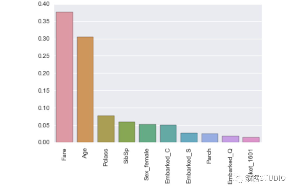
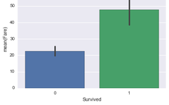
From the above figure, we can see that fare and age are important features. We can further examine the distribution of survival versus non-survival with respect to fare:

sns.barplot(y_train, X_train['Fare'])

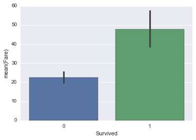
We can clearly see that survivors had a much higher average fare compared to non-survivors, so it seems reasonable to consider fare as an important feature.

Feature importance can be a good way to understand general feature significance. If a scenario arises where the model predicts that a passenger with a high fare would not survive, we can conclude that high fare does not necessarily lead to survival. Next, we will analyze other features that might lead the model to predict that this passenger would not survive.

This individual-level analysis can be very useful for production machine learning systems. Consider other examples, such as using the model to predict whether someone can receive a loan. We know that credit score will be a very important feature for the model, but what if there is a customer with a high credit score who gets rejected by the model? How do we explain this to the customer? And how do we explain it to the management?

Fortunately, recent research from the University of Washington on explaining the prediction processes of arbitrary classifiers has emerged. Their method is called LIME, which has been open-sourced on GitHub (https://github.com/marcotcr/lime). This article does not intend to delve into this topic, and you can refer to the paper (https://arxiv.org/pdf/1602.04938.pdf).

Next, we attempt to apply LIME in the model. Essentially, we first need to define an interpreter that handles the training data (we need to ensure that the training dataset passed to the interpreter is indeed the dataset that will be trained):

X_train_imputed = cv.best_estimator_.named_steps['imputer'].transform(X_train)
explainer = lime.lime_tabular.LimeTabularExplainer(X_train_imputed, 
    feature_names=X_train.columns.tolist(),
    class_names=["Not Survived", "Survived"],
    discretize_continuous=True)

Then, you must define a function that takes a feature array as input and returns an array with the probabilities for each class:

model = cv.best_estimator_.named_steps['model']
def xgb_prediction(X_array_in):
    if len(X_array_in.shape) < 2:
        X_array_in = np.expand_dims(X_array_in, 0)
    return model.predict_proba(X_array_in)

Finally, we pass an example and let the interpreter use your function to output feature values and labels:

X_test_imputed = cv.best_estimator_.named_steps['imputer'].transform(X_test)
exp = explainer.explain_instance(
      X_test_imputed[1], 
      xgb_prediction, 
      num_features=5, 
      top_labels=1)
exp.show_in_notebook(show_table=True, 
                     show_all=False)

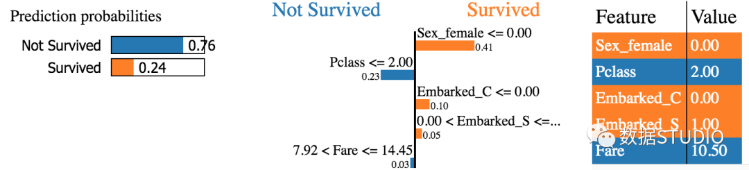
Here we have an example where there is a 76% probability of not surviving. We also want to see which features contribute the most to each class and how important they are. For example, survival probability is higher when Sex = Female. Let’s take a look at the bar chart:

sns.barplot(X_train['Sex_female'], y_train)

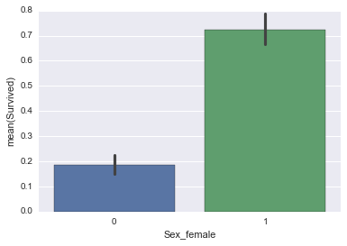
So this makes sense. If you are female, it significantly increases your chances of survival in the training data. So why is the prediction result “not survived”? It seems that Pclass = 2.0 greatly reduces the survival rate. Let’s take a look:

sns.barplot(X_train['Pclass'], y_train)

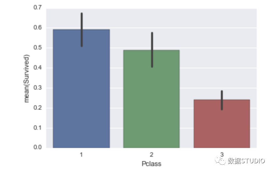
It seems that the survival rate for Pclass equal to 2 is still relatively low, so we have gained more understanding of our prediction results. Looking at the top 5 features displayed in LIME, it seems that this person should have survived, let’s take a look at the label:

y_test.values[0]>>>1

This person did survive, so our model is wrong! Thanks to LIME, we have some insight into the reasons for the issue: it seems that Pclass may need to be discarded. This approach can help us, and we hope to find some ways to improve the model.

This article provides readers with a simple and effective way to understand XGBoost. We hope these methods can help you make good use of XGBoost and enable your models to make better inferences.

Source: https://blogs.ancestry.com/