0. Introduction
After reading many blog posts and tutorials about RNN online, I felt they were all the same, providing a vague understanding but failing to explain it clearly. RNN is the foundation of many complex models, and even in transformers, you can see the influence of RNN, so it is essential to have a clear understanding of this model.
1. Why RNN is Needed
This brings us to the issues with CNN. Firstly, the characteristic of CNN is unidirectional propagation, meaning that the features within the same layer are independent. Additionally, the input layer of CNN requires fixed-length features. For example, if the input layer has 100 units, then the features fed into the model must also be 100. It is challenging to process additional input information.
Generally, CNN is good at handling 2D image data, abstracting and summarizing the implicit features of images. However, in the real world, there are many quantities that change over time, such as temperature variations over a year, physiological signals from the human body, and data outputs from gyroscopes. These belong to time series data, with the main characteristic of time series data being temporal correlation, where data points are related over time. Thus, we hope to have a model that can consider (remember) the characteristics of past data, which is where RNN comes into play.
2. The Simplest RNN Model
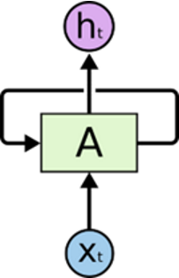
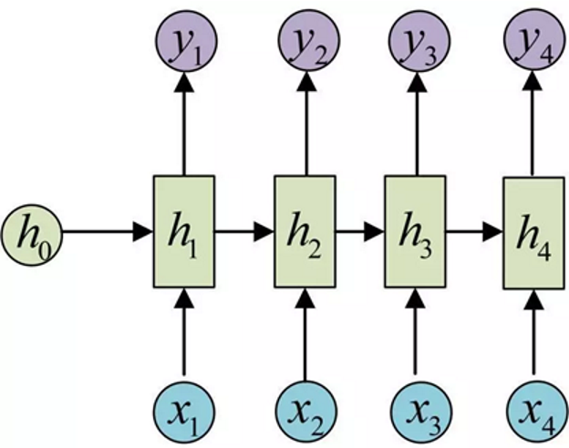
I’m sure everyone has seen many images similar to the ones below online. They are highly abstracted and simplified diagrams. The left image is very simple, but I felt confused after looking at it. When I look at the right image, which expands over time, I see an initial state h0, followed by four inputs x1 to x4, representing four time steps in the time series. x1-x4 are the input features, which are generally a vector or matrix. Of course, it could also just be a single value, but I still don’t understand what this h is all about. Let’s look further.
The formula provided by the PyTorch official website:
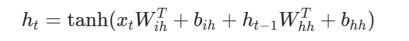
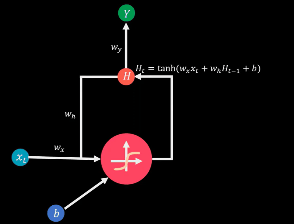
From the formula, we can see that the input featuresXt after passing through the neural network output as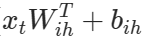 . The output ht-1 from the previous time step xt-1 also goes through the neural network, outputting as
 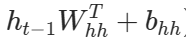 . Adding these two items together and applying tanh() for activation results in the current ht. This cycle continues, forming the recurrent neural network.
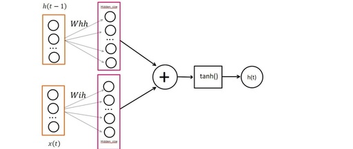
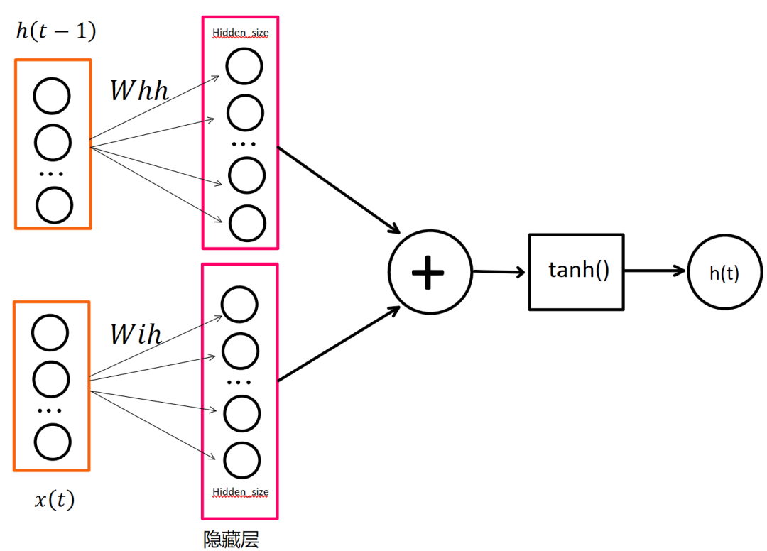
Looking at the image below, it is clear that Wih represents the weight parameters input to the neural network, associated with the input, hence the ‘i’. Whh is the weight parameters from the hidden layer to the neural network, marked with ‘h’. b is the bias. ht-1 and xt are both inputs to the neural network, multiplied by their respective weight coefficients, and added to the bias, which is the standard neuron operation process, just with an additional step of summation and activation. The value of h is related to the past, serving as a memory.
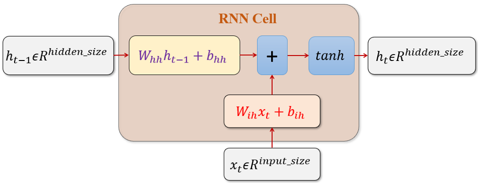
To provide a more intuitive understanding, the image below illustrates the details. It is important to note that the diagram below depicts two hidden layers, but in reality, there is only one, which is reused at different time steps. However, each weight matrix is different, so the results after hidden layer operations will also differ. The image below shows the computation process of a single step in RNN. Understanding this diagram will definitely help in grasping RNN.
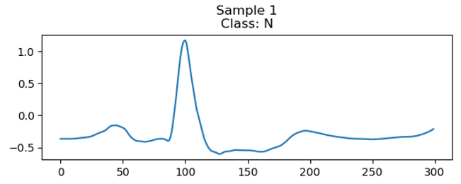
The dimensionality of the input feature x is determined by the input data. For example, climate changes can use wind speed, temperature, humidity, etc., as input features. If it is an electrocardiogram signal, then the input would be a single value of the collected surface potential. As shown in the image below, the sequence length of the electrocardiogram signal is 300, meaning there are 300 time steps, with each time step having only one value, so the input feature dimension is 1.
The number of neurons in the hidden layer is defined by hidden_size. Naturally, the more neurons there are, the greater the computational load.
Now we can explain why RNN can handle variable-length inputs.
Carefully observe theanimated graphic below. For natural language, each word corresponds to an input feature, and they can be input sequentially, regardless of the length of the sentence, which does not matter too much, it is just a matter of feeding data multiple times.
However, the computational complexity of RNN is linearly related to the sequence length (time step length).
RNN can have more than one hidden layer, but generally not more than three layers.
3. Bidirectional RNN
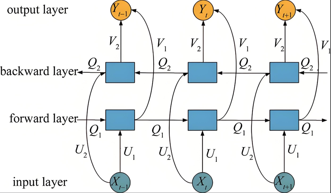
The RNN structure model described above can only observe past information, but future data does not participate, which is why the bidirectional RNN structure was created. Essentially, the input feature sequence is reversed, and a backward propagation layer (hidden layer) is added to the model, combining the results of the computation with the forward output as the final output. For example, if the number of neurons in our hidden layer is 25, then the output result for each time step will have 25+25=50 data points.
When we extract the output from the last time step, the features here should be correlated with all input features, addressing the temporal correlation issue of time series data. If we need to perform classification, we can simply add a fully connected layer afterward.
4. Important Parameters
First, let’s look at the model definition for RNN on the PyTorch official website
class torch.nn.RNN(self, input_size, hidden_size, num_layers=1, nonlinearity='tanh', bias=True, batch_first=False, dropout=0.0, bidirectional=False, device=None, dtype=None)
There are several important parameters:
input_size – Dimension of the input features
hidden_size – Number of neurons in the hidden layer
num_layers – Number of hidden layers, default is 1
nonlinearity – Activation function 'tanh' or 'relu'. Default: 'tanh'
bias – Bias, default: True
dropout – Used to prevent overfitting, default: 0, meaning no dropout
bidirectional – Whether to use bidirectional RNN
Now let’s look at an example. This RNN model receives the aforementioned electrocardiogram signal, which has 300 sampling data points, meaning 300 time steps, with each input feature being only one:
class RnnModel(nn.Module):
    def __init__(self):
        super(RnnModel, self).__init__()
        '''
        Parameter explanation: (Input dimension, Hidden layer dimension, Number of layers)
        Input dimension(input_size): The size of each x input, i.e., the number of features for each x
        Hidden layer(hidden_size): Number of neurons in the hidden layer
        Number of layers (num_layers): Number of hidden layers
        '''
        self.rnn = nn.RNN(1, 50, 1, nonlinearity='tanh', batch_first=True)
        self.linear = nn.Linear(50, 5)
    def forward(self, x):
        r_out, h_state = self.rnn(x)
        output = self.linear(r_out[:, -1, :])
        return output
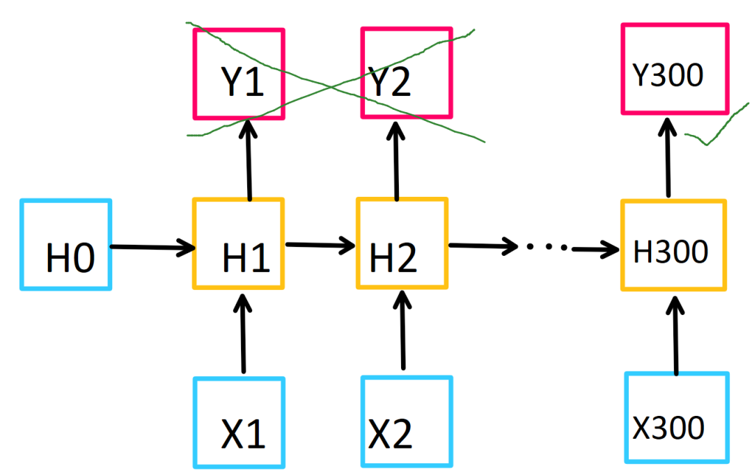
This RNN model feeds the model data one at a time, with 300 sampling values, so the RNN will loop 300 times for computation. Each step will produce an output, and since there are 50 neurons, the output result is also 50-dimensional. However, we only take the output value from the last time step and feed it into the fully connected layer for 5-class output. According to the diagram below, we extract Y300, which contains 50 features, establishing a neural network mapping from 50 to 5, achieving 5-class output.
5. Conclusion
With the foundational understanding of the RNN model above, you can quickly grasp and use many variants of the RNN model, such as LSTM, GRU, etc.