Implementing Adversarial Images and Attacks with Keras and TensorFlow

Author: Adrian Rosebrock

Translated by: Wu Zhendong

Proofread by: Zhang Damin

This article is about 8000 words, and it is recommended to read for 10+minutes. This article will tell you how to use image-based adversarial attacks to disrupt deep learning models, leveraging the Keras and TensorFlow deep learning libraries to implement your own adversarial attacks.[ Abstract ] In this tutorial, you will learn how to use image-based adversarial attacks to disrupt deep learning models. We will utilize the Keras and TensorFlow deep learning libraries to implement our own adversarial attacks.

Imagine twenty years from now. All vehicles on the road are autonomous vehicles powered by artificial intelligence, deep learning, and computer vision. Every turn, lane change, acceleration, and braking is supported by deep neural networks. Now, imagine yourself on a highway, sitting in the “driver’s seat” (can the driver’s seat still be called that when the car is self-driving?), with your wife in the passenger seat and your kids in the back seat. Looking ahead, you see a huge sticker on the lane where the vehicle is traveling, which seems to have no impact on the car’s forward motion. It looks like a popular large graffiti artwork, perhaps placed there by a few high school students as a joke, or maybe they just wanted to complete some big adventure game.

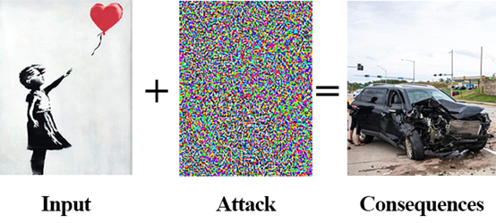
Figure 1: Executing an adversarial attack requires an input image (left), deliberately disturbed by a noise vector (middle), forcing the neural network to misclassify the input image, ultimately resulting in an incorrect classification, which could lead to serious consequences (right).In an instant, your car suddenly slams on the brakes and immediately changes lanes because that sticker on the road might depict a pedestrian, an animal, or another car. You are jolted in your seat, feeling like your neck is injured. Your wife screams, and the kids’ snacks bounce up in the back seat, splattering on the dashboard after hitting the windshield. You and your family are safe, but everything that just happened seems terrible.What happened? Why did your self-driving vehicle react this way? Is there some strange “bug” in the code or software inside the car? The answer is that the deep neural network supporting the vehicle’s visual component saw an adversarial image. Adversarial images are images that contain deliberately or intentionally disturbed pixels to confuse or deceive the model. Yet, at the same time, this image looks harmless and benign to humans. These images cause deep neural networks to intentionally make incorrect predictions. Adversarial images interfere with the model in such a way that they cannot make correct classifications. In fact, humans may not be able to visually distinguish between normal images and adversarial attack images — essentially, these two images look the same to the naked eye. This may not be an accurate (or correct) analogy, but I like to explain adversarial attacks in the context of image cryptography. Using cryptographic algorithms, we can embed data (such as plaintext information) into an image without changing the appearance of the image itself. This image can be sent to the receiver, who can then extract the hidden information from the image. Similarly, adversarial attacks embed a piece of information into the input image, but this information is not a plaintext message that people can understand because what is embedded in the input image by the adversarial attack is a noise vector. This noise vector is deliberately constructed to fool or confuse deep learning models. How do adversarial attacks work? How should we defend against them? In this tutorial, as well as in other posts in this series, we will accurately answer these questions. If you want to learn how to use Keras/TensorFlow to disrupt deep learning models with adversarial attacks and images, please continue reading. Implementing Adversarial Images and Attacks with Keras and TensorFlowIn the first part of this tutorial, we will discuss what adversarial attacks are and how they affect deep learning models.After that, we will implement three independent Python scripts:

1. The first Python script is a helper that loads the ImageNet dataset and parses category labels.
2. The second Python script utilizes a pre-trained ResNet model on the ImageNet dataset to perform basic image classification (demonstrating “standard” image classification).
3. The final Python script executes an adversarial attack and constructs an adversarial image that deliberately confuses our ResNet model, while these two images look the same to the naked eye.

Let’s get started! What are adversarial objects and adversarial attacks? How do they affect deep learning models?

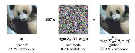
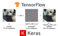
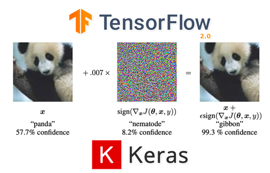
Figure 2: When performing an adversarial attack, the neural network is given an image (left), then a noise vector is constructed using gradient descent (middle). This noise vector is added to the input image, generating a misclassification (right). In 2014, Goodfellow et al. published a paper titled “Explaining and Harnessing Adversarial Examples” demonstrating the appealing property of deep neural networks — the potential to deliberately disrupt an input image, leading the neural network to misclassify it. This disruption is known as an adversarial attack. A classic example of an adversarial attack is illustrated in Figure 2 above. On the left, our input image is classified as a “panda” by the neural network with a confidence of 57.7%. In the middle, there is a noise vector that appears random to the human eye, but in fact is anything but. On the contrary, the pixels in this noise vector “equal the sign of the gradient of the loss function of the input image” (Goodfellow et al.). Embedding this noise vector into the input image produces the output shown in Figure 2 (right). To us, this new image looks exactly the same as the input image, but our neural network classifies this image as a “gibbon” with a confidence of 99.7%. Strange, right? A Brief History of Adversarial Attacks and Adversarial Images

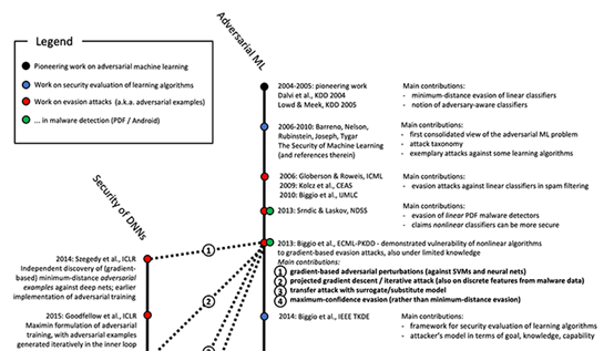
Figure 3: A timeline of publications on adversarial machine learning and the security of deep neural networks (Image source: Can Machine Learning Be Secure? Figure 8) Adversarial machine learning is not a new field, and these attacks are not exclusive to deep neural networks. In 2006, Barreno et al. published a paper titled “Can Machine Learning Be Secure?” discussing adversarial attacks and proposing some defenses against them. Back in 2006, the state-of-the-art machine learning models included Support Vector Machines (SVMs) and Random Forests (RFs), both of which are vulnerable to adversarial attacks. With the rise of deep neural networks in 2012, there was hope that these nonlinear models would not be easily affected by such attacks, yet Goodfellow et al. shattered that illusion. They found that deep neural networks are as susceptible to adversarial attacks as their predecessors. If you want to learn more about the history of adversarial attacks, I recommend checking out the paper “Wild Patterns: Ten Years After the Rise of Adversarial Machine Learning” by Biggio and Roli published in 2017. Why are Adversarial Attacks and Adversarial Images a Problem?

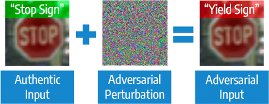
Figure 4: Why are adversarial attacks a problem? Why should we care? (Image source: imagesource) The example discussed at the top of this tutorial outlines why adversarial attacks can pose serious risks to our health, lives, and property. Other consequences are less severe, such as a group of hackers identifying a model used by Google for filtering spam in Gmail or recognizing a Facebook model for automatically detecting NSFW (not safe for work) content. If these hackers wanted to bypass Gmail’s spam filter to overload users with resources, or bypass Facebook’s NSFW filter to upload a large amount of pornographic content, theoretically they could do so. These are examples of minor consequences caused by adversarial attacks. Scenarios involving severe consequences could include hackers or terrorists identifying the deep neural networks used by self-driving cars worldwide (imagine if Tesla monopolized the market and became the only manufacturer of self-driving cars). Adversarial images could potentially be strategically placed on lanes or roads, causing chain accidents, property damage, or injuries to passengers, or even fatalities. Only your imagination, the extent of your knowledge about known models, and how they are used is the ceiling for adversarial attacks. Can We Defend Against Adversarial Attacks?The good news is that we can reduce the impact of adversarial attacks (but we cannot eliminate them entirely). This topic will not be covered in today’s tutorial but may be discussed in future tutorials. Setting Up Your Development EnvironmentTo set up your system for this tutorial, I recommend following these two tutorials:

• How to Install TensorFlow 2.0 on Ubuntu?
• How to Install TensorFlow 2.0 on macOS?

These two tutorials will assist you in configuring your system with the necessary software in a convenient Python virtual environment.Project Structure:

$ tree --dirsfirst.├── pyimagesearch│ ├── __init__.py│ ├── imagenet_class_index.json│ └── utils.py├── adversarial.png├── generate_basic_adversary.py├── pig.jpg└── predict_normal.py1 directory, 7 files

In the pyimagesearch module, there are two files:

1. imagenet_class_index.json: A JSON file that maps ImageNet category labels to readable strings. We will use this JSON file to determine the integer value index of a set of special labels, which will assist us in constructing adversarial image attacks.
2. utils.py: Contains simple Python helper functions for loading and parsing imagenet_class_index.json

There are also two Python scripts we need to check today:

1. predict_normal.py: Receives an input image (pig.jpg), loads the ResNet50 model, and classifies the input image. The output of this script will be the predicted category label index in ImageNet.
2. generate_basic_adversary.py:Using the output from the predict_normal.py script, we will construct an adversarial attack to fool ResNet, and the output (adversarial.png) will be stored on the hard disk.

Are you ready to implement your first adversarial attack in Keras and TensorFlow? Let’s get started. ImageNet Class Label/Index Helper UtilityBefore we begin executing normal image classification or adversarial attack using confused image classification, we first need to create a Python helper function to load and parse the category labels of the ImageNet dataset. We provide a JSON file containing all category label indices, identifiers, and readable strings, all contained in the project directory structure in the pyimagesearch module’s imagenet_class_index.json file. Here are the first few lines of the JSON file:

{"0": ["n01440764","tench"],"1": ["n01443537","goldfish"],"2": ["n01484850","great_white_shark"],"3": ["n01491361","tiger_shark"],..."106": ["n01883070","wombat"],...

As you can see, this file is in dictionary format. The dictionary’s keys are the integer value indices of category labels, while the values consist of binary tuples:

1. The unique identifier for the ImageNet label;
2. The human-readable category label.

Our goal is to implement a Python function that can parse the JSON file:

1. Receive an input label;
2. Convert it into its corresponding category label integer value index.

Essentially, we are transforming the key and value relationship in the imagenet_class_index.json file. Let’s implement this helper function. Open the utils.py file in the pyimagesearch module and insert the following code:

# import necessary packagesimport jsonimport osdef get_class_idx(label):# build the path to the ImageNet class label mappings filelabelPath = os.path.join(os.path.dirname(__file__), "imagenet_class_index.json")

Lines 2 and 3 import the Python packages we need. We will use the json Python module to load the JSON file, while the os package is used to construct the file path, which does not depend on what operating system you are using. Next, we define the get_class_idx helper function. The purpose of this function is to receive an input category label and obtain the integer value index of the predicted label (i.e., the prediction made by the model trained on ImageNet across 1000 category labels). Line 7 constructs the path to load the imagenet_class_index.json in the pyimagesearch module. Now load the contents of the JSON file:

# open the ImageNet class mappings file and load the mappings as# a dictionary with the human-readable class label as the keyand# the integer index as the valuewith open(labelPath) as f:imageNetClasses = {labels[1]: int(idx) for (idx, labels) in json.load(f).items()}# check to see if the input class label has a corresponding# integer index value, and if so return it; otherwise return# a None-type value return imageNetClasses.get(label, None)

In lines 4-6, we open the labelPath file and transform the key-value relationship of the pairs so that the keys are readable label strings, while the values are the integer value indices of those labels. To obtain the integer value index of the input label, we can call the .get method on the imageNetClasses dictionary (the last line), which will return:

• If the label exists in the dictionary, it returns the integer value index of that label;
• Otherwise, it returns None.

This value is returned to the calling function. Let’s build the get_class_idx helper function in the next section. Image Classification without Adversarial Attacks using Keras and TensorFlowAfter implementing the ImageNet class label/index helper function, let’s construct an image classification script that performs basic classification without adversarial attacks. This script can demonstrate that our ResNet model performs normally (makes correct predictions). In the latter part of this tutorial, you will find out how to construct an adversarial image to confuse ResNet. Let’s start with the basic image classification script — open the predict_normal.py file in your project structure and insert the following code:

# import necessary packagesfrom pyimagesearch.utils import get_class_idxfrom tensorflow.keras.applications import ResNet50from tensorflow.keras.applications.resnet50 import decode_predictionsfrom tensorflow.keras.applications.resnet50 import preprocess_inputimport numpy as npimport argparseimport imutilsimport cv2

In lines 2-9, we import the necessary Python packages. If you have used Keras, TensorFlow, and OpenCV before, these should be familiar to you. If you are new to Keras and TensorFlow, I strongly recommend checking out my tutorial “Keras Tutorial: How to Get Started with Keras, Deep Learning, and Python“. Additionally, you might want to read my book “Deep Learning for Computer Vision with Python” to deepen your understanding of training custom neural networks. In line 2, we import the get_class_idx function defined in the previous section, which can obtain the integer index value of the highest predicted label in the ResNet50 model. Let’s define the preprocess_image helper function:

def preprocess_image(image):# swap color channels, preprocess the image, and add in a batch# dimensionimage = cv2.cvtColor(image, cv2.COLOR_BGR2RGB)image = preprocess_input(image)image = cv2.resize(image, (224, 224))image = np.expand_dims(image, axis=0)# return the preprocessed imagereturn image

The preprocess_image method takes a single required parameter, which is the image we want to preprocess. Preprocessing this image involves the following steps:

1. Convert the image’s BGR channel combination to RGB;
2. Execute the preprocess_input function to complete the special preprocessing and scaling process in ResNet50;
3. Resize the image to 224×224;
4. Add a batch dimension.

This preprocessed image will be returned to the calling function. Next, let’s parse the command-line arguments:

# construct the argument parser and parse the argumentsap = argparse.ArgumentParser()ap.add_argument("-i", "--image", required=True, help="path to input image")args = vars(ap.parse_args())

We only need one command-line argument, –image, which is the path to the input image stored on the hard disk. If you have never dealt with command-line arguments and argparse before, I suggest checking out this tutorial. Next, load the input image and preprocess it:

# load image from disk and make a clone for annotationprint("[INFO] loading image...")image = cv2.imread(args["image"])output = image.copy()# preprocess the input imageoutput = imutils.resize(output, width=400)preprocessedImage = preprocess_image(image)

We load the input image using cv2.imread. In line 4, we make a copy of this image so we can later draw boxes on the output and annotate it with the predicted category label. We resize the output image to have a width of 400 pixels to fit our computer screen. Here we also use the preprocess_image function to process it into an input image suitable for classification by ResNet. Now, let’s load ResNet and classify the image:

# load the pre-trained ResNet50 modelprint("[INFO] loading pre-trained ResNet50 model...")model = ResNet50(weights="imagenet")# make predictions on the input image and parse the top-3 predictionsprint("[INFO] making predictions...")predictions = model.predict(preprocessedImage)predictions = decode_predictions(predictions, top=3)[0]

In line 3, we load the ResNet model with pre-trained weights on the ImageNet dataset. In lines 6 and 7, we make predictions on the preprocessed image, then decode the predictions using the decode_predictions helper function in Keras/TensorFlow. Now let’s see the top 3 (highest confidence) categories predicted by the neural network and display the category labels:

# loop over the top three predictionsfor (i, (imagenetID, label, prob)) in enumerate(predictions):# print the ImageNet class label ID of the top prediction to our# terminal (we'll need this label for our next script which will# perform the actual adversarial attack)if i == 0:print("[INFO] {} => {}".format(label, get_class_idx(label)))# display the prediction to our screenprint("[INFO] {}.{}: {:.2f}%".format(i + 1, label, prob * 100))

In line 2, we start a loop over the top-3 predicted results. If this is the first predicted result (i.e., the top-1 prediction), we display the readable label in the terminal, and then use the get_class_idx function to find the corresponding integer value index for that label in ImageNet. We can also display the top-3 labels and their corresponding probability values in the terminal. The final step is to annotate the top-1 predicted result on the output image:

# draw the top-most predicted label on the image along with the# confidence scoretext = "{}:{:.2f}%".format(predictions[0][1], predictions[0][2] * 100)cv2.putText(output, text, (3, 20), cv2.FONT_HERSHEY_SIMPLEX, 0.8, (0, 255, 0), 2)# show the output imagecv2.imshow("Output", output)cv2.waitKey(0)

The output image is displayed in the terminal, and if you click the OpenCV window or press any key, the output image will close. Non-Adversarial Image Classification ResultsNow we can perform basic image classification (non-adversarial attack) using ResNet. First, obtain the source code and image examples from the “Download” page. From here, open a terminal and execute the following command:

$ python predict_normal.py --image pig.jpg[INFO] loading image...[INFO] loading pre-trained ResNet50 model...[INFO] making predictions...[INFO] hog => 341[INFO] 1. hog: 99.97%[INFO] 2. wild_boar: 0.03%[INFO] 3. piggy_bank: 0.00%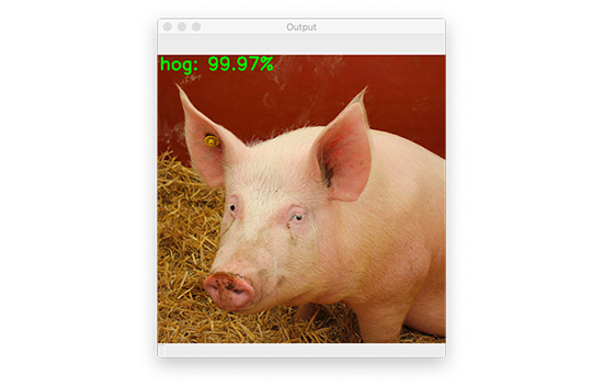

Figure 5: The pre-trained ResNet model correctly classifies this image as a “hog”. Here you can see we classified an image of a pig with a confidence of 99.97%. Additionally, we have included the ID for the hog label (341). We will use this label ID in the next chapter, where we will perform an adversarial attack on this input image of a pig. Implementing Adversarial Images and Attacks with Keras and TensorFlowNext, we will learn how to implement adversarial images and adversarial attacks with Keras and TensorFlow. Open the generate_basic_adversary.py file and insert the following code:

# import necessary packagesfrom tensorflow.keras.optimizers import Adamfrom tensorflow.keras.applications import ResNet50from tensorflow.keras.losses import SparseCategoricalCrossentropyfrom tensorflow.keras.applications.resnet50 import decode_predictionsfrom tensorflow.keras.applications.resnet50 import preprocess_inputimport tensorflow as tfimport numpy as npimport argparseimport cv2

In lines 2-10, we import the necessary Python packages. You will notice we again use the ResNet50 architecture, as well as the corresponding preprocess_input function (for preprocessing/scaling the input image) and decode_predictions for decoding the prediction output and displaying readable ImageNet labels. SparseCategoricalCrossentropy is used to calculate the classification cross-entropy loss between the label and prediction values. By using the sparse version of categorical cross-entropy, we do not need to one-hot encode class labels like we would with scikit-learn’s LabelBinarizer or Keras/TensorFlow’s to_categorical function. For example, in the predict_normal.py script, we have the preprocess_image function, and we will need it in this script as well:

def preprocess_image(image):# swap color channels, resize the input image, and add a batch# dimensionimage = cv2.cvtColor(image, cv2.COLOR_BGR2RGB)image = cv2.resize(image, (224, 224))image = np.expand_dims(image, axis=0)# return the preprocessed imagereturn image

Other than omitting the call to the preprocess_input function, this code segment is the same as the previous one, and you will soon understand why we omit calling that function when we start creating adversarial images. Next, we have a simple helper function, clip_eps:

def clip_eps(tensor, eps):# clip the values of the tensor to a given range and return itreturn tf.clip_by_value(tensor, clip_value_min=-eps, clip_value_max=eps)

The purpose of this function is to accept an input tensor and clip the input to the value range [-eps, eps]. The clipped tensor will be returned to the calling function. Now let’s look at the generate_adversaries function, which is the soul of the adversarial attack:

def generate_adversaries(model, baseImage, delta, classIdx, steps=50):# iterate over the number of stepsfor step in range(0, steps):# record our gradients with tf.GradientTape() as tape:# explicitly indicate that our perturbation vector should# be tracked for gradient updates tape.watch(delta)

The generate_adversaries method is the core of this entire script. This function takes four required parameters and a fifth optional parameter:

1. model: The ResNet50 model (if you prefer, you can swap it for another pre-trained model, such as VGG16, MobileNet, etc.);
2. baseImage: The original, unperturbed input image, for which we intentionally create an adversarial attack that causes the model to misclassify it.
3. delta: The noise vector that will be added to the baseImage, ultimately leading to misclassification. We will use the gradient descent mean to update this delta vector.
4. classIdx: The integer value index of the category label obtained from the predict_normal.py script.
5. steps: The number of steps for gradient descent (default is 50 steps).

Starting from line 3, we loop over the specified number of steps. Next, we use GradientTape to record the gradient. We call the .watch method on the tape to indicate that the perturbation vector can be used to track updates. Now we can construct the adversarial image:

# add our perturbation vector to the base image and# preprocess the resulting imageadversary = preprocess_input(baseImage + delta)# run this newly constructed image tensor through our# model and calculate the loss with respect to the# *original* class indexpredictions = model(adversary, training=False)loss = -sccLoss(tf.convert_to_tensor([classIdx]), predictions)# check to see if we are logging the loss value, and if# so, display it to our terminalif step % 5 == 0:print("step: {}, loss: {}...".format(step, loss.numpy()))# calculate the gradients of loss with respect to the# perturbation vectorgradients = tape.gradient(loss, delta)# update the weights, clip the perturbation vector, and# update its valueoptimizer.apply_gradients([(gradients, delta)])delta.assign_add(clip_eps(delta, eps=EPS))# return the perturbation vectorreturn delta

In line 3, we add the delta perturbation vector to the baseImage to construct the adversarial image, and the resulting image will be passed through the ResNet50’s preprocess_input function for scaling and normalization of the resulting adversarial image. The meaning of the next few lines is:

• In line 7, we use the model parameter’s imported model to make predictions on the newly created adversarial image.
• In lines 8 and 9, we calculate the loss with respect to the original class index (classIdx, obtained from running predict_normal.py).
• In lines 12-14, we display the loss value every 5 steps.

In line 17, outside the with statement, we calculate the gradient of the loss with respect to the perturbation vector. Next, we can update the delta vector, clipping off values that exceed the range of [-EPS, EPS]. Finally, we return the obtained perturbation vector to the calling function — that is, the final delta value that allows us to construct the adversarial attack to deceive the model. After the core implementation of the adversarial script, the next step is to parse the command-line arguments:

# construct the argument parser and parse the argumentsap = argparse.ArgumentParser()ap.add_argument("-i", "--input", required=True, help="path to original input image")ap.add_argument("-o", "--output", required=True, help="path to output adversarial image")ap.add_argument("-c", "--class-idx", type=int, required=True, help="ImageNet class ID of the predicted label")args = vars(ap.parse_args())

Our adversarial attack Python script requires three command-line arguments:

1. –input: The disk path to the input image (e.g., pig.jpg);
2. –output: The path to the output adversarial image (e.g., adversarial.png);
3. –class-idx: The integer value index of the category label in the ImageNet dataset. We can obtain this index by executing the predict_normal.py mentioned in the “Non-Adversarial Image Classification Results” section.

Next, we initialize a few variables and load/preprocess the –input image:

# define the epsilon and learning rate constantsEPS = 2 / 255.0LR = 0.1# load the input image from disk and preprocess itprint("[INFO] loading image...")image = cv2.imread(args["input"])image = preprocess_image(image)

In line 2, we define the epsilon value (EPS) used to clip the tensor when constructing the adversarial image. 2 / 255.0 is a standard value for EPS used in adversarial publications or tutorials (if you want to learn more about default values, you can refer to this guide). In line 3, we define the learning rate. As a rule of thumb, the initial value for LR is generally set to 0.1, and you may need to adjust this value when creating your own adversarial images. The last two lines load the input image and preprocess it using the preprocess_image helper function. Next, we can load the ResNet model:

# load the pre-trained ResNet50 model for running inferenceprint("[INFO] loading pre-trained ResNet50 model...")model = ResNet50(weights="imagenet")# initialize optimizer and loss functionoptimizer = Adam(learning_rate=LR)sccLoss = SparseCategoricalCrossentropy()

In line 3, we load the ResNet50 model trained on the ImageNet dataset. We will use the Adam optimizer and sparse categorical loss to update our perturbation vector. Now let’s construct the adversarial image:

# create a tensor based off the input image and initialize the# perturbation vector (we will update this vector via training)baseImage = tf.constant(image, dtype=tf.float32)delta = tf.Variable(tf.zeros_like(baseImage), trainable=True)# generate the perturbation vector to create an adversarial exampleprint("[INFO] generating perturbation...")deltaUpdated = generate_adversaries(model, baseImage, delta, args["class_idx"])# create the adversarial example, swap color channels, and save the# output image to diskprint("[INFO] creating adversarial example...")adverImage = (baseImage + deltaUpdated).numpy().squeeze()adverImage = np.clip(adverImage, 0, 255).astype("uint8")adverImage = cv2.cvtColor(adverImage, cv2.COLOR_RGB2BGR)cv2.imwrite(args["output"], adverImage)

In line 3, we construct a tensor based on the input image, and in line 4, we initialize the perturbation vector delta. We can call the generate_adversaries function using the ResNet50 model, the input image, the initialized perturbation vector, and the integer value index of the class label to update the delta vector. During the execution of the generate_adversaries function, the delta perturbation vector will be continuously updated, generating the final noise vector deltaUpdated. In the second to last line, we add the deltaUpdated vector to the baseImage to create the final adversarial image (adverImage). Then, we perform the following three post-processing steps on the generated adversarial image:

1. Clip values that exceed the range of [0, 255];
2. Convert the image to an unsigned 8-bit integer (so OpenCV can process the image);
3. Convert the channel order from RGB to BGR.

After these processing steps, we can write the adversarial image to the hard disk. The real question is, can our newly created adversarial image deceive our ResNet model? The next piece of code will answer this question:

# run inference with this adversarial example, parse the results,# and display the top-1 predicted resultprint("[INFO] running inference on the adversarial example...")preprocessedImage = preprocess_input(baseImage + deltaUpdated)predictions = model.predict(preprocessedImage)predictions = decode_predictions(predictions, top=3)[0]label = predictions[0][1]confidence = predictions[0][2] * 100print("[INFO] label: {} confidence: {:.2f}%".format(label, confidence))# draw the top-most predicted label on the adversarial image along# with the confidence scoretext = "{}: {:.2f}%".format(label, confidence)cv2.putText(adverImage, text, (3, 20), cv2.FONT_HERSHEY_SIMPLEX, 0.5, (0, 255, 0), 2)# show the output imagecv2.imshow("Output", adverImage)cv2.waitKey(0)

In line 4, we create another adversarial image, still by adding the delta noise vector to the original input image, but this time we process it using ResNet’s preprocess_input function. The generated preprocessed image goes into ResNet, and we obtain the top-3 predicted results and decode them (lines 5 and 6). Next, we obtain the top-1 label and its corresponding probability/confidence and display these values in the terminal (lines 7-10). The final step is to annotate the highest predicted value on the output adversarial image and display it on the screen.Results of Adversarial Images and AttacksAre you ready to witness an adversarial attack? From here, you can open a terminal and execute the following code:

$ python generate_basic_adversary.py --input pig.jpg --output adversarial.png --class-idx 341[INFO] loading image...[INFO] loading pre-trained ResNet50 model...[INFO] generating perturbation...step: 0, loss: -0.0004124982515349984...step: 5, loss: -0.0010656398953869939...step: 10, loss: -0.005332294851541519...step: 15, loss: -0.06327803432941437...step: 20, loss: -0.7707189321517944...step: 25, loss: -3.4659299850463867...step: 30, loss: -7.515471935272217...step: 35, loss: -13.503922462463379...step: 40, loss: -16.118188858032227...step: 45, loss: -16.118192672729492...[INFO] creating adversarial example...[INFO] running inference on the adversarial example...[INFO] label: wombat confidence: 100.00%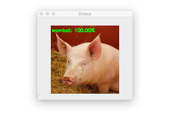

Figure 6: Previously, this input image was correctly classified as “hog”, but now due to the adversarial attack, it has been classified as “wombat”!

Our input image pig.jpg was previously classified as “hog”, but now its label has become “wombat”! Let’s compare the original image and the adversarial image generated by the generate_basic_adversary.py script:

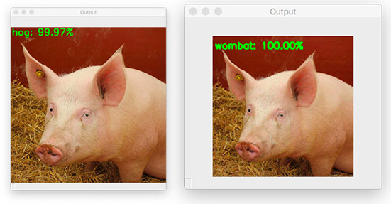
Figure 7: On the left is the original image, with the classification result being correct. On the right is the adversarial image, which has been incorrectly classified as “wombat”. To the human eye, there is no discernible difference between the two images. On the left is the original image of the pig, and on the right is the output adversarial image, which has been misclassified as “wombat”. As you can see, these two images have no perceivable differences; our human eyes cannot discern any difference, but for ResNet, they are indeed completely different. This is great, but we cannot clearly control the final category label recognized by the adversarial image. This raises the following question:Can we control the final category label of the input image? The answer is yes, and this will be the topic of my next tutorial. In summary, adversarial images and adversarial attacks are indeed thought-provoking. But when we see the next tutorial, we will be able to preemptively defend against this type of attack. More details will be provided later.AcknowledgmentsIf it weren’t for the work of Goodfellow, Szegedy, and other deep learning researchers, this tutorial would not have been possible. Additionally, the implementation code used in this tutorial was inspired by the official TensorFlow implementation of “Fast Gradient Signed Method“. I strongly recommend checking out other examples; each code segment is more explicit in theory and mathematics than what is presented in this tutorial. ConclusionIn this tutorial, you learned about adversarial attacks, how they work, and as artificial intelligence and deep neural networks become more integrated with the world, adversarial attacks will pose a greater threat.Next, we implemented a basic adversarial attack algorithm using the deep learning libraries Keras and TensorFlow.With adversarial attacks, we can deliberately disrupt an input image, for example:

1. This input image will be misclassified.
2. However, the perturbation image still looks the same to the naked eye.

Using the methods employed in this tutorial, we cannot control the final category label that the image is ultimately classified as — we are simply creating a noise vector and embedding it into the input image, causing the deep neural network to misclassify it.What if we could control the final category label? For instance, if we take an image of a “dog” and create an adversarial attack to make the convolutional neural network think it is an image of a “cat”, is that possible?The answer is yes — we will discuss this topic in the next tutorial.Original link:https://www.pyimagesearch.com/2020/10/19/adversarial-images-and-attacks-with-keras-and-tensorflow/Original title:Adversarial images and attacks with Keras and TensorFlow——END——