Source: Algorithm Advancement


This article is approximately 4800 words long and is suggested to be read in 8 minutes.
This article introduces the functionality of neural networks.
In the fields of machine learning and related areas, artificial neural networks are computational models inspired by biological neural networks: each neuron is connected to other neurons, and when it is excited, it sends chemical substances to neighboring neurons, thereby altering the potential within those neurons; if the potential of a certain neuron exceeds a threshold, it will be activated (excited) and send chemical substances to other neurons.
Artificial neural networks are typically presented as “neurons” connected in a structured hierarchy, allowing for distributed parallel information processing algorithms based on input computational values. This network relies on the complexity of the system, adjusting the relationships between a large number of interconnected nodes to achieve information processing. It is also used to estimate or rely on a large amount of input and generally unknown approximating functions to maximize the fit of actual data in reality, improving the accuracy of machine learning predictions.
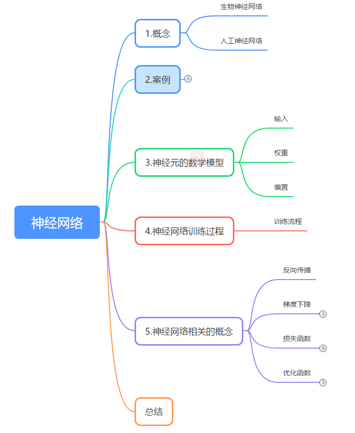
Simply discussing the concept of neural networks can be somewhat abstract, so let’s first demonstrate the complete process of data processing using neural networks in machine learning through an example.
1.1 Case Introduction
Example: Train a neural network model to fit the relationship between advertising investment (TV, radio, newspaper – 3 methods) and sales output (sales), in order to predict sales based on advertising expenditure.
Sample data:
https://github.com/justmarkham/scikit-learn-videos/blob/master/data/Advertising.csv
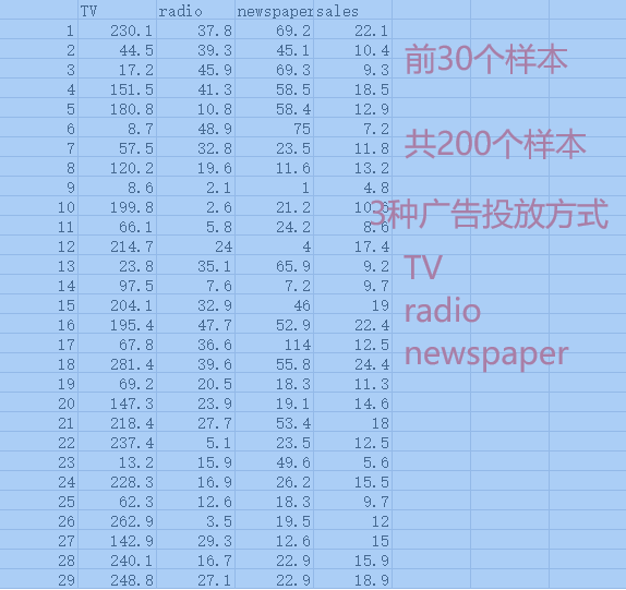
Sample Data
TV, radio, and newspaper are the 3 features of the sample data, while sales is the sample label.
# Importing libraries
import tensorflow as tf
import pandas as pd
import numpy as np

# Loading data
data = pd.read_csv('../dataset/Advertising.csv')
# pd is the data analysis library pandas
# Building model to predict sales based on TV, radio, and newspaper investment
print(type(data),data.shape)###<class 'pandas.core.frame.DataFrame'> (200, 5)

# Extracting features x excluding the first and last columns
x = data.iloc[:,1:-1] # 200*3
# Extracting label y from the last column
 y = data.iloc[:,-1] # 200*1
1.3 Building a Neural Network
Establishing a Sequential model:
Hidden layer: a multi-layer perceptron (10 layers Dense(10), shape input_shape=(3,), corresponding to the 3 feature columns of the sample, activation function activation=”relu”)
Output layer: label is a predicted value, dimension is 1
model = tf.keras.Sequential([
tf.keras.layers.Dense(10,input_shape=(3,),activation="relu"),
tf.keras.layers.Dense(1)])
Model structure print(model.summary())
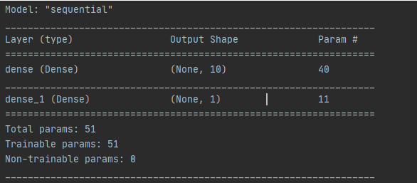
1) keras model, Sequential indicates a sequential model, as it is fully connected, we choose a sequential model
2) tf.keras.layers.Dense is the API for adding network layers
3) Hidden layer parameters: 40, 10 perceptrons (neurons), each perceptron has 4 parameters (w1,w2,w3,b), totaling 10*4 = 40
4) Output layer parameters: 11, 1 perceptron (neuron), parameters (w1,w2,w3,w4,w5,w6,w7,w8,w9,w10,b) totaling 11
5) Total number of model parameters: 40+11 = 51
1.4 Adding Optimizer and Loss Function to the Created Model
# Optimizer adam, linear regression model loss function is mean squared error (mse)
model.compile(optimizer="adam",loss="mse")
1.5 Starting Training
model.fit(x,y,epochs=100)
x is the sample features; y is the sample labels
epochs is a concept in gradient descent, when a complete dataset has passed through the neural network once and returned, this process is called one epoch; when one epoch is too large for the computer, it needs to be divided into smaller batches, which will be detailed in the following gradient descent section.
1.6 Using the Model for Prediction
# Using the model to predict the sales of the first 10 samples in the existing data
test = data.iloc[:10,1:-1]
print('Test values',model.predict(test))
The above steps demonstrate the entire process of building, training, and predicting a neural network model. Next, we will introduce the principles.
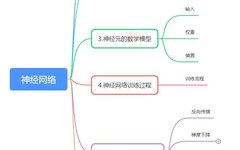
2 Mathematical Model of Neurons
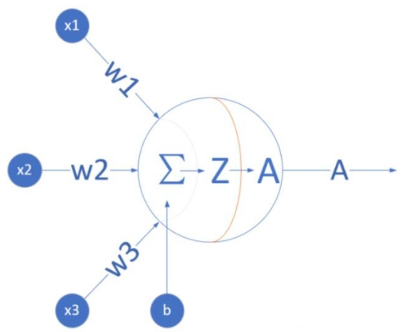
Mathematical Model of Neurons
(x1, x2, x3) are the external input signals, generally multiple attributes/features of a training data sample, which can be understood as the 3 advertising expenditure methods in the example.
(w1,w2,w3) are the weight values of each input signal, for the example of (x1,x2,x3), x1’s weight might be 0.92, x2’s weight might be 0.2, and x3’s weight might be 0.03. Of course, the sum of the weight values may not equal 1.
Where does b come from? Generally, books or blogs will tell you it is because y=wx+b; b is the offset value that allows the line to move up and down along the Y-axis. From a biological perspective, in brain neural cells, the neuron will only be excited when the level/current of the input signal exceeds a certain threshold, and this b is actually that threshold. That is, when: w1*x1+w2*x2+w3*x3>=t, the neuron will be excited. We move t to the left side of the equation, turning it into (−t), and then write it as b, resulting in: w1*x1+w2*x2+w3*x3+b>=0
3 Training Process of Neural Networks
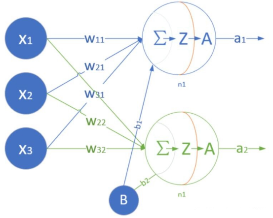
Using the previous advertising expenditure as an example, before training a neural network, a network needs to be built, then filled with data (adding sample data containing features and labels) for training. The training process involves continuously updating weights w and biases b. There are 10 layers of input, and the number of features in each layer is determined by the samples (the 3 feature columns of the advertising expenditure in the example). Each layer has 4 parameters (w1,w2,w3,b), and for a fully connected network with 10 layers, that amounts to 10*4=40 parameters. Below is a single-layer neural network model, but with 2 neurons.
The training process involves continuously updating weights w and biases b until stable w and b are found that minimize the overall error of the model. The specific process is as follows:
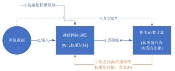
Illustration of Training Process
4 Concepts Related to Neural Networks
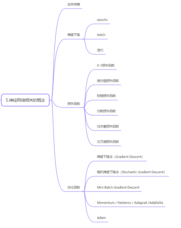
4.1 Backpropagation
The backpropagation algorithm is an efficient technique for calculating gradients in data flow graphs; the derivative of each layer is the product of the derivative of the next layer and the output from the previous layer, which is the beauty of the chain rule that the error backpropagation algorithm utilizes.
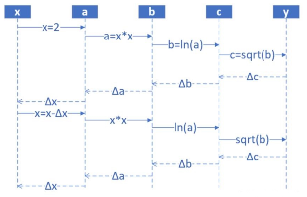
Illustration of Backpropagation Algorithm
During feedforward, starting from the input, each hidden layer’s output is calculated sequentially until the output layer.
Step 1: Input layer, randomly input the first x value, with x ranging from (1,10], suppose x is 2;
Step 2: First layer network calculation, receives x value from step 1, calculates: a=x^2;
Step 3: Second layer network calculation, receives a value from step 2, calculates: b=ln (a);
Step 4: Third layer network calculation, receives b value from step 3, calculates: c=sqrt{b};
Step 5: Output layer, receives c value from step 4
Then begin calculating the derivatives, and backpropagate from the output layer through each hidden layer sequentially. To reduce computation, all computed elements need to be reused.
Backpropagation — The derivative of each layer is the product of the derivative of the next layer and the output from the previous layer
Step 6: Calculate the difference between y and c: Δc = c-y, passing it back to step 4
Step 7: Step 4 receives Δc from step 5, calculates Δb = Δc*2sqrt(b)
Step 8: Step 3 receives Δb from step 4, calculates Δa = Δb*a
Step 9: Step 2 receives Δa from step 3, calculates Δx = Δ/(2*x)
Step 10: Step 1 receives Δx from step 2, updates x (x-Δx), returns to step 1, and begins the next cycle from the input layer.
Gradient descent is an iterative optimization algorithm used in machine learning to find the best results (the minimum of a curve), which includes the following two meanings:
-
Gradient: The fastest ascent point of the function’s current position;
-
Descent: The opposite direction of the derivative, mathematically described as that negative sign, which means moving in the opposite direction of ascent, which is descent, reducing the cost function.
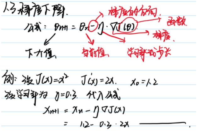
Mathematical Formula for Gradient Descent
-
-
-
-: Negative sign, the reverse of the gradient,
-
η: Learning rate or step size, controlling the distance of each step, not too fast to avoid missing extreme points; not too slow to prevent excessive convergence time
-
▽: Gradient, the fastest ascent point of the function’s current position
-
The gradient descent algorithm is iterative, meaning it requires multiple uses of the algorithm to obtain results, leading to optimal results. The iterative nature of gradient descent allows the underfitting graph to evolve to achieve the best fit for the data.
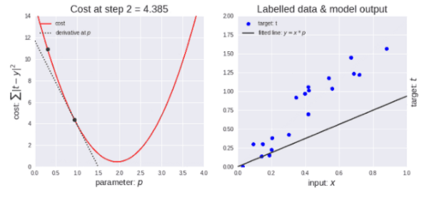
Illustration of Gradient Descent Algorithm
As shown in the left of the above image, initially, the learning rate is large, thus the descent step is larger. As the point descends, the learning rate becomes smaller, thus the descent step also becomes smaller. Meanwhile, the cost function is decreasing, or the cost is decreasing, which is sometimes referred to as the loss function, both are the same.
In general, it is impossible to input the entire dataset into the computer at once. Therefore, to solve this problem, we need to divide the data into smaller chunks and pass them to the computer one at a time, updating the neural network’s weights at the end of each step to fit the given data. This requires understanding concepts like epochs and batch size.
When a complete dataset has passed through the neural network once and returned, this process is called one epoch. However, when one epoch is too large for the computer, it needs to be divided into smaller chunks.
Setting the Number of Epochs
The complete dataset is passed multiple times through the same neural network. But remember, we are using a limited dataset and an iterative process, i.e., gradient descent, to optimize the learning process and visualization. Therefore, merely updating the weights once or using one epoch is not sufficient.

It is not enough to pass the complete dataset through the neural network once, and as the number of epochs increases, the number of updates to the weights in the neural network also increases, causing the curve to shift from underfitting to overfitting. So, how many epochs are appropriate? Well, there is no definite standard answer to this question; developers need to set it based on the characteristics of the dataset and personal experience.
When it is not possible to pass the data through the neural network all at once, the dataset needs to be divided into several batches.
Iteration is the number of times a batch needs to complete one epoch. Remember: in one epoch, the number of batches and iterations is equal.
For example, for a dataset with 2000 training samples, if the 2000 samples are divided into batches of size 400 (5 batches), then completing one epoch requires 5 iterations.
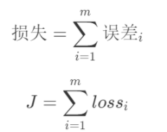
4.3 Loss Function
The “loss” is the total of the “errors” of all samples, i.e., (mm is the number of samples):
-
-
(2) Absolute Loss Function
-
-
-
(5) Mean Squared Error Loss Function
-
(6) Cross-Entropy Loss Function
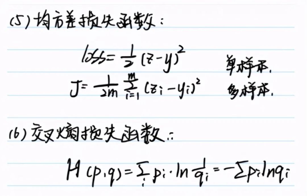
Mean Squared Error and Cross-Entropy Expressions
4.4 Optimization Functions
In section 1.4 of the example, an optimizer and loss function were added to the created model
# Optimizer adam, linear regression model loss function is mean squared error (mse)
model.compile(optimizer="adam",loss="mse")
Here, the Adam optimizer is used; there are many optimization methods in neural networks, and here are a few briefly introduced, detailed information needs to be looked up separately.
Gradient descent is the most important method and is the basis for many other optimization algorithms.
2) Stochastic Gradient Descent
Updates are made using only one sample at a time, which has a small computational load and high update frequency; it can easily lead to model overfitting and instability, as well as unstable convergence.
3) Mini Batch Gradient Descent
Mini-batch gradient descent is a compromise between gradient descent and stochastic gradient descent, where the loss is calculated for a batch rather than directly calculating the loss for the entire dataset or just one sample.
Gradient descent with momentum is also a commonly used optimization algorithm. This method accelerates gradient descent by introducing momentum.
The NAG algorithm, in short, performs a rehearsal before updating using momentum gradient descent to see if the update along the previous direction is appropriate; if not, it immediately adjusts the direction. This means that the direction of parameter updates is no longer the current gradient direction but the true direction the parameters should go in the future.
During training, each parameter has its learning rate, which decays based on its previous squared gradient.
Advantages: During training, there is no need to manually adjust the learning rate; generally, just set the default initial learning rate.
Disadvantages: As iterations progress, the learning rate in formula (6) becomes smaller due to the increasing denominator, leading to minimal updates in the model during the later training stages.
AdaDelta is an improved version of Adagrad, aimed at solving the issue of very small learning rates during the later stages of training, which slows down convergence.
Previously, we started with the classic gradient descent method and introduced several improved versions of gradient descent.
-
The Momentum method improves the convergence speed by adding momentum;
-
The Nesterov method finds a more suitable gradient direction and magnitude for the current situation by performing a rehearsal before updating;
-
Adagrad allows different parameters to have different learning rates and automatically reduces the learning rate during training by introducing the squared sum of gradients;
-
AdaDelta improves upon Adagrad to ensure a more suitable learning rate during the later stages of training.
Since different parameters can have different learning rates, can different parameters also have different momentums?
The Adam method is based on this idea, where each parameter not only has its learning rate but also its momentum value, allowing for more independent updates during training, improving model training speed and stability.
Adam (Adaptive Moment Estimation):
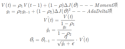
Generally, ρ1 is set to 0.9, and ρ2 is set to 0.999
To quote someone: Adam works well in practice and outperforms other Adaptive techniques.
In fact, if your data is sparse, methods like SGD, NAG, and Momentum often perform poorly because the same learning rate is used for different parameters in the model, leading to parameters that should update quickly updating slowly, while those that should update slowly may update quickly due to data reasons. Therefore, for sparse data, adaptive methods (Adagrad, AdaDelta, Adam) should be used. Similarly, for deep neural networks or very complex neural networks, using Adam or other adaptive methods can also lead to faster convergence.
5 Summary
Let’s review the main content of this article:
1) Understanding Concepts: Artificial neural networks are inspired by biological neural networks, and by increasing the number of hidden layer neurons, they can approximate any continuous function to enhance the model’s approximation accuracy.
2) The example introduced the process of constructing an artificial neural network model in machine learning.
3) The training process of artificial neural networks.
4) Detailed introduction to some basic concepts related to neural networks: backpropagation, gradient descent, loss functions, optimization functions, epochs, batch size, optimizers, learning rates, etc.
Editor: Wang Jing
Proofreader: Lin Yilin