Source: Machine Learning Algorithms Explained
Friends familiar with deep learning know that LSTM is a type of RNN model that can conveniently handle time series data and is widely used in fields such as NLP.
0. Starting from RNN
Recurrent Neural Network (RNN) is a type of neural network used to process sequential data. Compared to general neural networks, it can handle data that changes over sequences. For example, the meaning of a word may differ based on the preceding context, and RNN can effectively address such issues.
1. Ordinary RNN
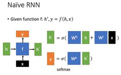
Let’s briefly introduce a typical RNN. Its main form is shown in the figure below (all images are from Professor Li Hongyi’s PPT):
is the input data at the current state, represents the input received from the previous node.
is the output at the current node state, andis the output passed to the next node.
From the formula in the above figure, we can see that the output h’ is related to both x and h.
y is often calculated from h’ by passing it into a linear layer (mainly for dimensional mapping) and then using softmax for classification to obtain the required data.
The specific method of how y is derived from h’ often depends on the model’s usage.

2. LSTM
2.1 What is LSTM
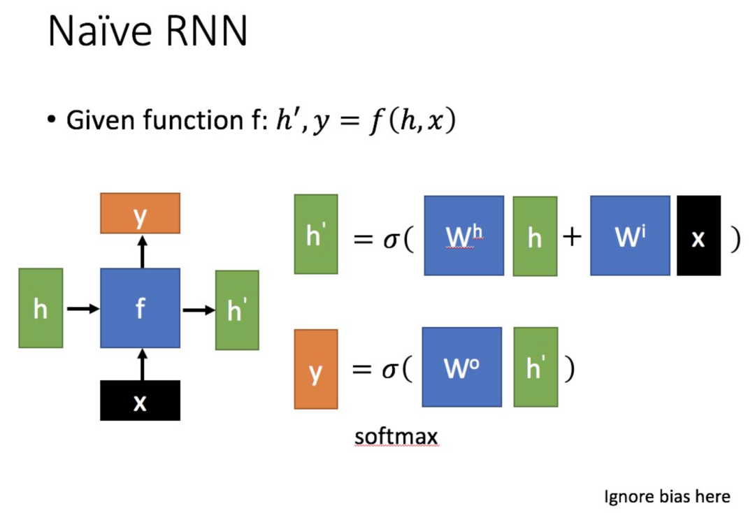
Long Short-Term Memory (LSTM) is a special type of RNN, primarily designed to address the problems of gradient vanishing and gradient explosion during the training of long sequences. In simple terms, compared to ordinary RNNs, LSTM performs better over longer sequences.
The structure of LSTM (right image) differs from that of ordinary RNN in terms of input and output as shown below.
Compared to RNN, which only has one state to pass, LSTM has two states: one (cell state) and one (hidden state). The state in RNN is equivalent to the state in LSTM.
For the state that is passed along, it changes very slowly; typically, the output is the previous state plus some values.
Meanwhile, often varies significantly across different nodes.
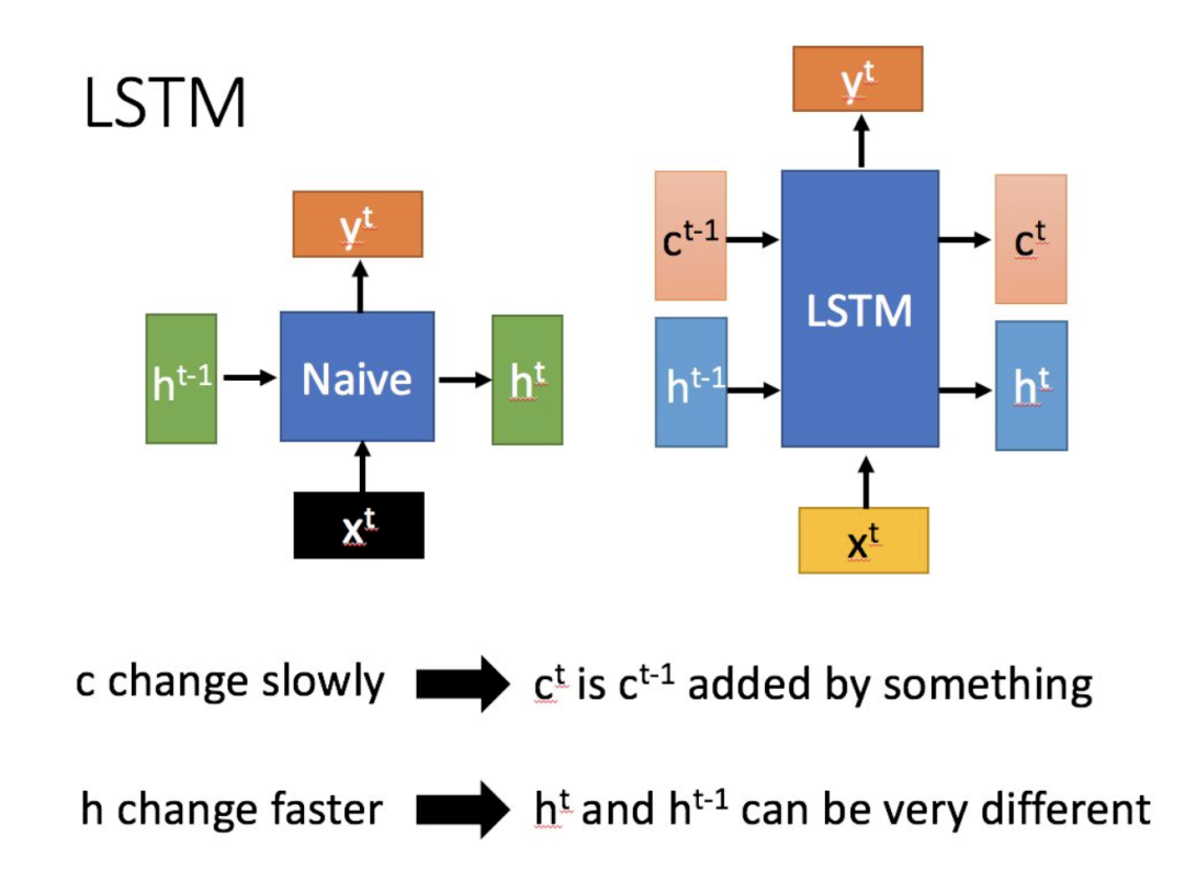
2.2 Delving into LSTM Structure
Next, we will specifically analyze the internal structure of LSTM.
First, by using the current input and the previous state , we concatenate them to train and obtain four states.

Where , , is obtained by multiplying the concatenated vector by a weight matrix and then passing it through a sigmoid activation function to convert it into a value between 0 and 1, serving as a gating state. While is transformed to a value between -1 and 1 using a tanh activation function (here tanh is used because it serves as input data, not a gating signal).
Now, let’s further introduce how these four states are utilized internally in LSTM (note this down)
represents the Hadamard Product, which means multiplying corresponding elements in the matrices, thus requiring the two matrices to be of the same shape. denotes matrix addition.
There are three main stages within LSTM:
1. Forgetting Stage. This stage mainly performs selective forgetting on the input from the previous node. In simple terms, it will “forget the unimportant, remember the important.”
Specifically, this is controlled by the forget gate calculated as (f represents forget) to determine which parts of the previous state should be retained and which should be forgotten.
2. Selective Memory Stage. This stage selectively “remembers” the current input. It focuses on recording important inputs while downplaying the less important ones. The current input is represented by the previously calculated . The gating signal for selection is controlled by (i represents information).
The results obtained from the above two steps can be summed up to get the state that will be passed to the next state, which is the first formula in the above image.
Similar to ordinary RNNs, the output is often derived from the transformation of .
3. Conclusion
In summary, this is the internal structure of LSTM. It uses gating states to control the transmission states, remembering what needs to be remembered for a long time, and forgetting the unimportant information; unlike ordinary RNNs, which can only “naively” accumulate memory in one way. This is particularly useful for many tasks that require “long-term memory.”
However, due to the introduction of many elements, it leads to an increase in parameters and makes training considerably more challenging. Therefore, we often use GRU, which has similar performance to LSTM but fewer parameters, to build models for large training volumes.