This article is approximately 3900 words long and is recommended for an 8-minute read.
In this article, we demonstrate that Causal Attention can be rewritten in the form of an RNN.
In recent years, RNNs have rekindled interest among researchers and users due to their linear training and inference efficiency, hinting at a “Renaissance” in the field, with notable works including RWKV [1], RetNet [2], and Mamba [3]. When RNNs are used for language modeling, their typical characteristics include constant space complexity and linear time complexity for each step of generation, resulting in constant space complexity and linear time complexity for the entire sequence.
Of course, everything has two sides. Compared to the dynamically growing KV cache of Attention, the constant space complexity of RNNs often raises doubts about their limited memory capacity, making it difficult for them to compete with Attention on long contexts.
In this article, we show that Causal Attention can be rewritten in the form of RNN, and that its generation at each step can theoretically also achieve constant space complexity (at the cost of a significantly higher time complexity, far exceeding quadratic levels). This indicates that the advantages of Attention (if any) are built on computation rather than intuitively expanded memory; like RNNs, they fundamentally possess a constant order memory capacity (memory bottleneck).
Supporters of RNNs often present a seemingly irrefutable argument: Think about whether your brain is more like an RNN or Attention?
Intuitively, the space complexity of RNN inference is constant, while the KV cache of Attention grows dynamically. Considering that human brain capacity is limited, one must admit that RNNs are indeed closer to the human brain from this perspective.
However, even if it is reasonable to believe that brain capacity limits the space complexity of each step of reasoning to be constant, it does not limit the time complexity of each step to be constant. In other words, even if the time complexity of each step for humans is constant, when processing a sequence of length L, humans may not only scan the sequence once (e.g., “flipping through a book”), leading to a total number of reasoning steps that may significantly exceed L, resulting in nonlinear time complexity.
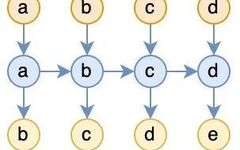
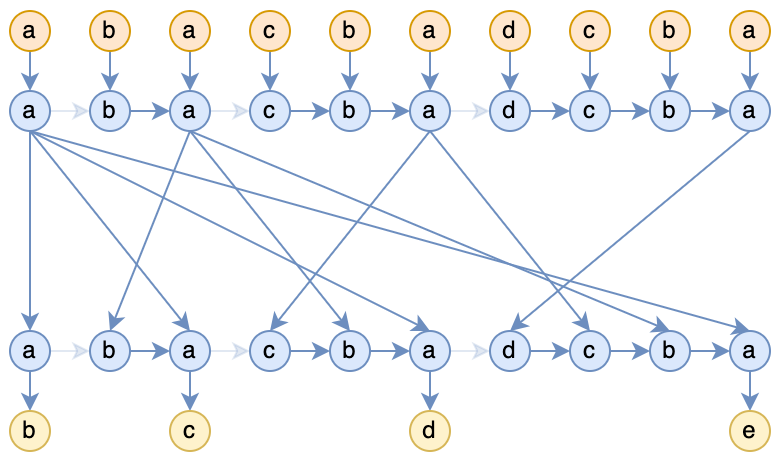
Considering this, the author had a “eureka” moment: is it possible to generalize a model of RNN with constant space complexity and nonlinear time complexity to supplement the capabilities that mainstream RNNs lack (such as the aforementioned book-flipping)? For language modeling tasks, assuming the sample is a b c d e, the training task is to input a b c d and predict b c d e, a common RNN is illustrated in the following diagram:
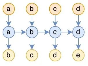
The problem with this RNN is that it lacks the ability to flip through books; each input is discarded after being read. In contrast, the characteristic of Attention is that for each token read, it completely revisits the history. Although this approach may have efficiency issues, it undoubtedly is the simplest and most straightforward way to introduce the book-flipping capability. To provide RNNs with this ability, we can completely mimic the approach of Attention:
Figure 2: RNN that continuously “flips through books”
Like Attention, each time a new token is read, the entire history is revisited. Of course, it can also be said that this does not design a new RNN but is merely a new usage of RNNs, simply modifying the input; both RWKV and Mamba can be applied here. Under this usage, decoding can still be completed within constant space complexity, but the time complexity of each inference step grows linearly, leading to a total time cost of .
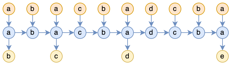
In fact, the model represented by Figure 2 is very broad, and Attention is only a special case of it, as shown in the following diagram:
Figure 3: RNN corresponding to Causal Attention
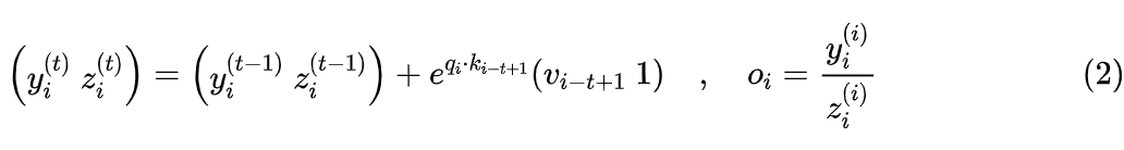
Compared to Figure 2, Figure 3 has several arrows blurred, indicating that these positions are actually disconnected, so Attention is merely a special case of Figure 2. Specifically, the computation formula for Attention is:
Clearly, both the numerator and denominator sums can be expressed recursively:
According to the literature I have read, the earliest work that proposed the above formula and used it to optimize Attention computation is “Self-attention Does Not Need O(n^2) Memory” [4], and the block matrix version of the above formula is the theoretical basis of the current mainstream acceleration technology Flash Attention. In Self Attention, since Q, K, and V are all obtained from the same input through token-wise operations, the above recursive form can just be represented as Figure 3.
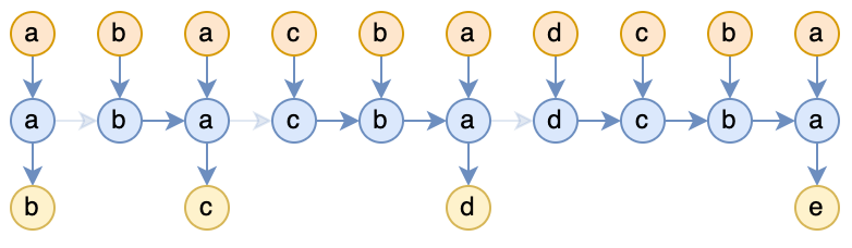
Of course, Figure 3 only depicts a single layer of Attention; multiple layers can naturally be drawn, but the connections may appear a bit complex, as shown in the following diagram for two layers:
Figure 4: RNN corresponding to two layers of Attention
03 Constant Space Complexity
As mentioned at the beginning of this article, the common advantage of RNNs is that they can perform inference with constant space complexity and linear time complexity. Since Attention can also be expressed as RNN, a natural question arises: does it also have these two advantages under this formulation?
Clearly, since the RNN corresponding to Attention has increased the sequence length to , linear time complexity is out of the question; the only thing worth pondering is whether it can achieve constant space complexity?
Everyone’s first reaction might be that it cannot, as it is well known that Attention decoding has a dynamically linear growing KV cache. However, this is just a more efficient implementation in typical cases. If we do not mind the cost of trading time for space, how much can space complexity be further reduced?
The answer may be surprising: if we truly push the trade-off of time for space to the extreme, we can indeed reduce the space complexity to !
This conclusion is not difficult to imagine. Firstly, the single-layer Attention shown in Figure 3 is essentially no different from an ordinary single-layer RNN, and thus can clearly perform inference using fixed-size storage space.
Next, let’s look at the multi-layer Attention shown in Figure 4. Its connections between layers are relatively complex, so it usually requires caching historical K and V to compute efficiently. However, if we resolutely do not store the KV cache, then the K and V for each layer and each step of inference can be recalculated completely from the original input (recomputation), leading to a lot of redundant calculations, resulting in a total time complexity that far exceeds quadratic complexity, which is very inefficient, but the space complexity can indeed be maintained at .
For example, in the case of two layers of Attention, the second layer of Attention uses the output of the first layer of Attention as input, and each output of the first layer of Attention can be computed within space, so as long as we are willing to sacrifice efficiency for recomputation, the second layer of Attention can also be completed within space.
Following this logic, the third layer of Attention uses the output of the second layer of Attention as input, and the Nth layer of Attention uses the output of the N-1 layer of Attention as input. Since the previous layer can be computed within space through recomputation, every layer and even the entire model can be computed within space.
This brings us back to the initial point of the article: if Attention does have any advantages over RNNs, it is merely achieved through more computation; the intuitive expansion of “memory” is just the appearance of trading space for time, and it has a fundamental memory bottleneck of constant capacity like RNNs.
Of course, some readers might think: is trading time for space not a common practice? This does not seem to be a valuable conclusion. Indeed, trading time for space is common, but it is not always feasible. In other words, not all problems can achieve a reduction in space complexity to , which is a common but non-trivial characteristic.
04 Reflection on Model Capabilities
The reason for pointing out this characteristic of Attention is not to actually use it for reasoning but to help us further think about the capability bottlenecks of Attention.
First, if we really want to get into the details, is actually incorrect; more strictly speaking, it should be , because the RNN with quadratic complexity needs to repeatedly scan the historical sequence, which requires storing at least L integer token IDs, meaning the required space is , and if L is sufficiently large, then will be larger than .
However, the here primarily refers to the minimum space required for the computation layers in LLMs, comparable to the hidden_state when used as RNN, which includes at least (hidden_size * num_layers * 2) components, while the space is reflected in the input and output. An intuitive analogy is to view Attention as a computer with infinite hard disk space and fixed memory, continuously reading data from the hard disk and performing computations in memory while writing results back to the hard disk.
We know that when the memory is large and the data being processed is small, we usually program more “indulgently,” even loading all data into memory, with the intermediate computation processes completely independent of the reading and writing of the hard disk.
Similarly, LLMs trained under the context of “large models, short sequences” are more likely to leverage the fixed “memory” brought by model scale, rather than the dynamic “hard disk” brought by sequence length, because under the current scale of LLMs, the former is sufficiently large, and SGD tends to “cut corners” by treating the model as a machine with infinite static memory for training (since memory is always sufficient for short sequences). However, the static memory of the model is limited, so for tasks that cannot be completed in space, models based on Attention cannot generalize to arbitrary lengths of input.
For example, if we want to compute the decimal representation of y using Attention for conditional modeling p(y|x), the training corpus is concatenated, calculating only the loss for y. Note that here y can be uniquely determined by the input x, so theoretically, it should achieve 100% accuracy. However, if there is no chain of thought (CoT) to dynamically increase the sequence length, the model can only implicitly place all computation processes in “memory,” which is always effective for short inputs.
However, memory is limited, and the space required for computation increases with x, so there must exist a sufficiently large x such that the accuracy of p(y|x) cannot reach 100% (even training accuracy). This is different from the length extrapolation problem discussed in “The Path to Transformer Upgrade: Re-examining Length Extrapolation Techniques”; it is not caused by OOD from positional encoding, but rather a capability defect brought about by training LLMs under the context of “large models, short sequences” without sufficient CoT guidance.
So why is the current mainstream scaling direction still to increase the memory of LLMs, i.e., to increase the hidden_size and num_layers, rather than to explore schemes like CoT that increase seq_len?
The latter is certainly one of the mainstream research directions, but the core issue is that if memory becomes a bottleneck, it will reduce the learning efficiency and universality of the model. Just as when memory is small and the data volume is large, we need to save results to the hard disk in a timely manner and clear the memory, which means algorithms must be more sophisticated, harder to write, and may even require customizing algorithm details based on specific tasks.
What situations lead to memory bottlenecks? Taking LLAMA2-70B as an example, its num_layers is 80, hidden_size is 8192, multiplying these gives 640K, and multiplying by 2 gives around 1M. In other words, when the input length reaches this level of 1M tokens, the “memory” of LLAMA2-70B may become a bottleneck. Although training LLMs at the 1M token level is still challenging, it is no longer out of reach; for example, Kimi has already launched internal testing of models at the 1M level.
Thus, continuously increasing the model’s context length (hard disk) to accommodate more input and CoT, while also scaling up the model itself to ensure that “memory” does not become a bottleneck, has become the current mainstream theme for LLMs.
This also negates a previous thought of mine: whether it is possible to achieve the same effect as large models by reducing model scale and increasing seq_len? The answer is likely no, because smaller models face memory bottlenecks; if they rely on the hard disk provided by seq_len, then sufficient long CoT must be set for each sample, which is more challenging than directly training large models. If seq_len is increased simply through repetition or other simple methods without introducing additional information, there will be no substantial benefit.
However, if increasing seq_len is achieved through prefix tuning, it may be possible to bridge the gap in space complexity, as the parameters of the prefix are not computed from the input sequence but are trained separately, effectively adding a series of “memory sticks” to increase the model’s memory.
05 The End of the Journey Through Space and Time
In this article, we examined Attention from the perspective of quadratic complexity RNNs and discovered its bottleneck of constant space complexity, indicating that Attention does not inherently increase “memory” compared to RNNs but merely increases the amount of computation. The existence of this bottleneck suggests that Attention may theoretically face difficulties in length generalization for certain tasks (due to insufficient memory). How to guide the model to better utilize the dynamic “hard disk” provided by seq_len dimensions may be the key to solving this difficulty.
[1] https://arxiv.org/abs/2305.13048
[2] https://arxiv.org/abs/2307.08621
[3] https://arxiv.org/abs/2312.00752
[4] https://arxiv.org/abs/2112.05682
Editor: Wang Jing