Understanding Learning Curves for XGBoost Models in Python

XGBoost is a powerful and efficient implementation of gradient boosting ensemble algorithms. Configuring the hyperparameters of the XGBoost model can be challenging, often leading to time-consuming and computationally intensive large grid search experiments. Another way to configure the XGBoost model is to evaluate the model’s performance at each iteration of the algorithm during training and plot the results as learning curves. These learning curve graphs provide a diagnostic tool that can be interpreted and suggest specific changes to the model’s hyperparameters that may improve predictive performance.

In this tutorial, you will learn how to plot and interpret the learning curves of XGBoost models in Python. By the end of this tutorial, you will know:

Learning curves provide a useful diagnostic tool for understanding the training dynamics of supervised learning models like XGBoost.
How to configure XGBoost to evaluate the dataset at each iteration and plot the results as learning curves.
How to interpret and use learning curve graphs to improve the performance of XGBoost models.

Tutorial Overview

This tutorial is divided into four parts. They are:

Extreme Gradient Boosting
Learning Curves
Plotting XGBoost Learning Curves
Using Learning Curves to Tune XGBoost Models

Extreme Gradient Boosting

Gradient boosting refers to a class of ensemble machine learning algorithms that can be used for classification or regression predictive modeling problems. The ensemble is built based on decision tree models. One tree is added to the ensemble at a time and adjusted to correct the prediction errors made by the previous models. This is a type of ensemble machine learning model known as Boosting. The model is fitted using any arbitrary differentiable loss function and gradient descent optimization algorithm. This gives the technique its name, “gradient boosting,” because the loss gradient is minimized as the model is fitted, very similar to neural networks.

Extreme Gradient Boosting (XGBoost) is an efficient open-source implementation of the gradient boosting algorithm. Therefore, XGBoost is an algorithm, an open-source project, and a Python library. It was originally developed by Tianqi Chen and described by Chen and Carlos Guestrin in their 2016 paper “XGBoost: A Scalable Tree Boosting System.” It is designed to be both computationally efficient (e.g., fast execution) and effective, perhaps more so than other open-source implementations. The two main reasons for using XGBoost are its execution speed and model performance. XGBoost dominates structured or tabular datasets in classification and regression predictive modeling problems. Evidence suggests it is the preferred algorithm of competition winners on the Kaggle data science platform.

Now that we understand what XGBoost is and why it is important, let’s take a closer look at learning curves.

Learning Curves

Typically, learning curves are graphs that display time or experience on the x-axis and learning or improvement on the y-axis.

Learning curves are widely used in algorithms in machine learning that learn gradually over time (optimizing their internal parameters), such as deep learning neural networks. The metrics used to evaluate learning may be maximized, meaning higher scores (larger numbers) indicate more learning. An example is classification accuracy.

More commonly, minimized scores are used, such as loss or error, where higher scores (smaller numbers) indicate more learning, with a value of 0.0 indicating that the model has learned well from the training dataset and has made no errors.

During the training process of a machine learning model, the current state of the model can be evaluated at each step of the training algorithm. It can be evaluated on the training dataset to understand how much the model has “learned.” It can also be evaluated on a hold-out validation dataset that does not belong to the training dataset. Evaluating on the validation dataset allows us to understand the model’s degree of “generalization.”

When training on both the training and validation datasets, dual learning curves are typically created for the machine learning model. The shape and dynamics of the learning curves can be used to diagnose the behavior of the machine learning model and, in turn, suggest types of configuration changes that could improve learning and/or performance.

You may observe three common dynamic changes in learning curves; they are:

Underfitting
Overfitting
Just Right Fitting

Most commonly, learning curves are used to diagnose a model’s overfitting behavior, which can be addressed by adjusting the model’s hyperparameters.

Overfitting refers to a model that learns too well from the training dataset, including statistical noise or random fluctuations in the training dataset. The problem with overfitting is that the more specialized the model is to the training data, the worse its ability to generalize to new data, leading to increased generalization error. The increase in generalization error can be measured by the model’s performance on the validation dataset.

Now that we are familiar with learning curves, let’s look at how to plot the learning curves for an XGBoost model.

Plotting XGBoost Learning Curves

In this section, we will plot the learning curves for an XGBoost model.

First, we need a dataset to fit and evaluate the model. In this tutorial, we will use a synthetic binary (two-class) classification dataset.

The make_classification() function from scikit-learn can be used to create a synthetic classification dataset. In this case, we will use 50 input features (columns) and generate 10,000 samples (rows). The seed for the pseudo-random number generator is fixed to ensure that the same base “problem” is used each time samples are generated.

The following example generates a synthetic classification dataset and summarizes the shape of the generated data.

# test classification dataset
from sklearn.datasets import make_classification
# define dataset
X, y = make_classification(n_samples=10000, n_features=50, n_informative=50, n_redundant=0, random_state=1)
# summarize the dataset
print(X.shape, y.shape)

Running the example will generate the data and report the size of the input and output components, confirming the expected shape.

(10000, 50) (10000,)

Next, we can fit the XGBoost model on this dataset and plot the learning curves. First, we need to split the dataset into a part that will be used to train the model (training), and another part that will not be used to train the model but will be held out and used to evaluate the performance of the model at each step of the training algorithm (test set or validation set).

# split data into train and test sets
X_train, X_test, y_train, y_test = train_test_split(X, y, test_size=0.50, random_state=1)

Then we can define the XGBoost classification model using the default hyperparameters.

# define the model
model = XGBClassifier()

Next, the model can be fitted to the dataset. In this case, we must specify the algorithm to evaluate the model’s performance on the training set and test the model on the test set at each iteration (e.g., after adding each new tree to the ensemble). To do this, we must specify the datasets to evaluate and the metrics to evaluate. The datasets must be specified as a list of tuples, where each tuple contains the input and output columns of the dataset, and each element in the list is a different dataset to evaluate, such as the training set and test set.

# define the datasets to evaluate each iteration
evalset = [(X_train, y_train), (X_test,y_test)]

We may want to evaluate many metrics, although given that this is a classification task, we will evaluate the model’s logarithmic loss (cross-entropy), which is a minimized score (the lower the value, the better).

This can be achieved by specifying the “eval_metric” parameter when calling fit() and providing the name of the metric we will evaluate, which will be “logloss”. We can also specify the datasets to evaluate via the “eval_set” parameter. The fit() function takes the training dataset as the first two parameters as usual.

# fit the model
model.fit(X_train, y_train, eval_metric='logloss', eval_set=evalset)

Once the model is fitted, we can evaluate its performance on the test dataset for classification accuracy.

# evaluate performance
yhat = model.predict(X_test)
score = accuracy_score(y_test, yhat)
print('Accuracy: %.3f' % score)

Then we can retrieve the metrics calculated for each dataset by calling the evals_result() function.

# retrieve performance metrics
results = model.evals_result()

This will return a dictionary organized first by dataset (“validation_0” and “validation_1”) and then by metric (“logloss”). We can create line plots of the metrics for each dataset.

# plot learning curves
pyplot.plot(results['validation_0']['logloss'], label='train')
pyplot.plot(results['validation_1']['logloss'], label='test')
# show the legend
pyplot.legend()
# show the plot
pyplot.show()

That’s it. In summary, here is the complete example of fitting an XGBoost model on a synthetic classification task and plotting the learning curves.

# plot learning curve of an xgboost model
from sklearn.datasets import make_classification
from sklearn.model_selection import train_test_split
from sklearn.metrics import accuracy_score
from xgboost import XGBClassifier
from matplotlib import pyplot
# define dataset
X, y = make_classification(n_samples=10000, n_features=50, n_informative=50, n_redundant=0, random_state=1)
# split data into train and test sets
X_train, X_test, y_train, y_test = train_test_split(X, y, test_size=0.50, random_state=1)
# define the model
model = XGBClassifier()
# define the datasets to evaluate each iteration
evalset = [(X_train, y_train), (X_test,y_test)]
# fit the model
model.fit(X_train, y_train, eval_metric='logloss', eval_set=evalset)
# evaluate performance
yhat = model.predict(X_test)
score = accuracy_score(y_test, yhat)
print('Accuracy: %.3f' % score)
# retrieve performance metrics
results = model.evals_result()
# plot learning curves
pyplot.plot(results['validation_0']['logloss'], label='train')
pyplot.plot(results['validation_1']['logloss'], label='test')
# show the legend
pyplot.legend()
# show the plot
pyplot.show()

Running the example fits the XGBoost model, retrieves the calculated metrics, and plots the learning curves.

Note: Due to the randomness of the algorithm or evaluation procedure, or differences in numerical precision, your results may vary. Consider running the example several times and comparing the average results.

First, the model performance is reported, indicating that the model achieved about 94.5% classification accuracy on the hold-out test set.

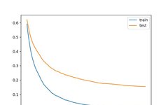
Accuracy: 0.945

The graph shows the learning curves for the training and test datasets, where the x-axis is the number of iterations of the algorithm (or the number of trees added to the ensemble), and the y-axis is the model’s logarithmic loss. Each line shows the logarithmic loss for each iteration for the given dataset. From the learning curves, we can see that the model’s performance on the training dataset (blue line) is better or has lower loss than the model’s performance on the test dataset (orange line), as we would typically expect.

Now that we know how to plot learning curves for XGBoost models, let’s see how to use these curves to improve model performance.

Using Learning Curves to Tune XGBoost Models

We can use learning curves as diagnostic tools. These curves can be interpreted and used as a basis for suggesting specific changes to the model configuration that may lead to better performance. The model and results from the previous section can serve as a baseline and starting point. Looking at the graph, we can see that both curves are trending downward, indicating that more iterations (adding more trees) may lead to further loss reduction. Let’s try that. We can increase the number of iterations by changing the “n_estimators” hyperparameter from the default of 100 to 500.

# define the model
model = XGBClassifier(n_estimators=500)

Here is the complete example:

# plot learning curve of an xgboost model
from sklearn.datasets import make_classification
from sklearn.model_selection import train_test_split
from sklearn.metrics import accuracy_score
from xgboost import XGBClassifier
from matplotlib import pyplot
# define dataset
X, y = make_classification(n_samples=10000, n_features=50, n_informative=50, n_redundant=0, random_state=1)
# split data into train and test sets
X_train, X_test, y_train, y_test = train_test_split(X, y, test_size=0.50, random_state=1)
# define the model
model = XGBClassifier(n_estimators=500)
# define the datasets to evaluate each iteration
evalset = [(X_train, y_train), (X_test,y_test)]
# fit the model
model.fit(X_train, y_train, eval_metric='logloss', eval_set=evalset)
# evaluate performance
yhat = model.predict(X_test)
score = accuracy_score(y_test, yhat)
print('Accuracy: %.3f' % score)
# retrieve performance metrics
results = model.evals_result()
# plot learning curves
pyplot.plot(results['validation_0']['logloss'], label='train')
pyplot.plot(results['validation_1']['logloss'], label='test')
# show the legend
pyplot.legend()
# show the plot
pyplot.show()

Running the example fits and evaluates the model and plots the learning curves for the model’s performance.

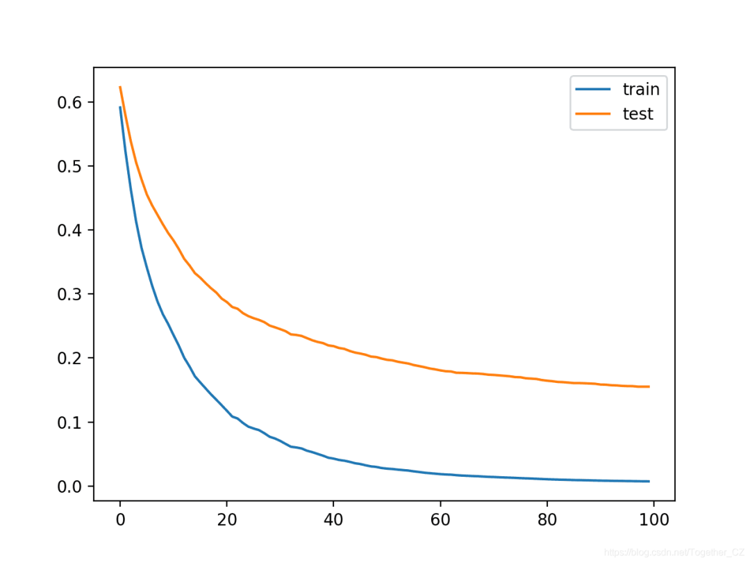
We can see that more iterations increased accuracy from about 94.5% to about 95.8%.

Accuracy: 0.958

From the learning curves, we can see that indeed, the additional iterations caused the curves to continue to decline, and then plateau after about 150 iterations, remaining at a reasonable level.

A longer flat curve may indicate that the algorithm is learning too quickly, and slowing down may be beneficial. This can be achieved using the learning rate, which limits the contribution of each tree added to the ensemble. This can be controlled by the “eta” hyperparameter, which has a default value of 0.3. We can try a smaller value, such as 0.05.

# define the model
model = XGBClassifier(n_estimators=500, eta=0.05)

Here is the complete example:

# plot learning curve of an xgboost model
from sklearn.datasets import make_classification
from sklearn.model_selection import train_test_split
from sklearn.metrics import accuracy_score
from xgboost import XGBClassifier
from matplotlib import pyplot
# define dataset
X, y = make_classification(n_samples=10000, n_features=50, n_informative=50, n_redundant=0, random_state=1)
# split data into train and test sets
X_train, X_test, y_train, y_test = train_test_split(X, y, test_size=0.50, random_state=1)
# define the model
model = XGBClassifier(n_estimators=500, eta=0.05)
# define the datasets to evaluate each iteration
evalset = [(X_train, y_train), (X_test,y_test)]
# fit the model
model.fit(X_train, y_train, eval_metric='logloss', eval_set=evalset)
# evaluate performance
yhat = model.predict(X_test)
score = accuracy_score(y_test, yhat)
print('Accuracy: %.3f' % score)
# retrieve performance metrics
results = model.evals_result()
# plot learning curves
pyplot.plot(results['validation_0']['logloss'], label='train')
pyplot.plot(results['validation_1']['logloss'], label='test')
# show the legend
pyplot.legend()
# show the plot
pyplot.show()

Running the example fits and evaluates the model and plots the learning curves for the model’s performance.

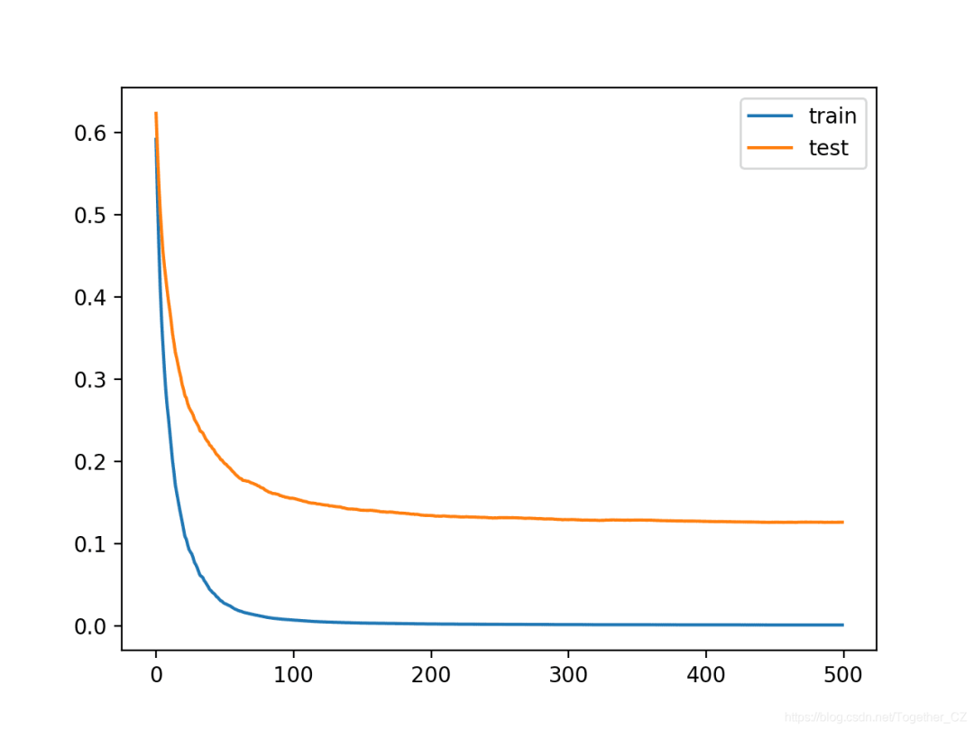
We can see that the smaller learning rate made the accuracy worse, dropping from about 95.8% to about 95.1%.

Accuracy: 0.951

From the learning curves, we can see that learning is indeed slowing down. The curves suggest that we could continue to add more iterations and might achieve better performance since the curves would have more opportunities to continue decreasing.

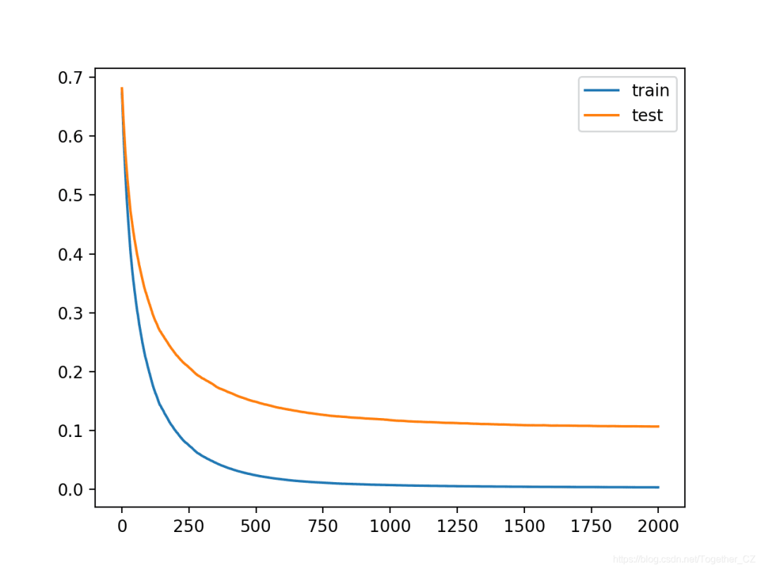
Let’s try increasing the number of iterations from 500 to 2,000.

# define the model
model = XGBClassifier(n_estimators=2000, eta=0.05)

Here is the complete example:

# plot learning curve of an xgboost model
from sklearn.datasets import make_classification
from sklearn.model_selection import train_test_split
from sklearn.metrics import accuracy_score
from xgboost import XGBClassifier
from matplotlib import pyplot
# define dataset
X, y = make_classification(n_samples=10000, n_features=50, n_informative=50, n_redundant=0, random_state=1)
# split data into train and test sets
X_train, X_test, y_train, y_test = train_test_split(X, y, test_size=0.50, random_state=1)
# define the model
model = XGBClassifier(n_estimators=2000, eta=0.05)
# define the datasets to evaluate each iteration
evalset = [(X_train, y_train), (X_test,y_test)]
# fit the model
model.fit(X_train, y_train, eval_metric='logloss', eval_set=evalset)
# evaluate performance
yhat = model.predict(X_test)
score = accuracy_score(y_test, yhat)
print('Accuracy: %.3f' % score)
# retrieve performance metrics
results = model.evals_result()
# plot learning curves
pyplot.plot(results['validation_0']['logloss'], label='train')
pyplot.plot(results['validation_1']['logloss'], label='test')
# show the legend
pyplot.legend()
# show the plot
pyplot.show()

Running the example fits and evaluates the model and plots the learning curves for the model’s performance.

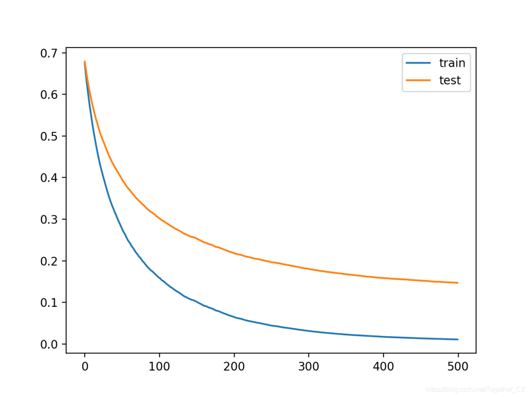
We can see that more iterations allowed the algorithm more room for improvement, achieving an accuracy of 96.1%, which is the best so far.

Accuracy: 0.961

The learning curves again show stable convergence of the algorithm, with sharp declines and long plateaus.

We can repeat the process of lowering the learning rate and increasing the number of iterations to see if it is possible to improve further. Another way to slow the learning speed is to add regularization in the form of reducing the number of samples and features (rows and columns) used to construct each tree in the ensemble. In this case, we will try to halve the number of samples and features using the “subsample” and “colsample_bytree” hyperparameters, respectively.

# define the model
model = XGBClassifier(n_estimators=2000, eta=0.05, subsample=0.5, colsample_bytree=0.5)

Here is the complete example:

# plot learning curve of an xgboost model
from sklearn.datasets import make_classification
from sklearn.model_selection import train_test_split
from sklearn.metrics import accuracy_score
from xgboost import XGBClassifier
from matplotlib import pyplot
# define dataset
X, y = make_classification(n_samples=10000, n_features=50, n_informative=50, n_redundant=0, random_state=1)
# split data into train and test sets
X_train, X_test, y_train, y_test = train_test_split(X, y, test_size=0.50, random_state=1)
# define the model
model = XGBClassifier(n_estimators=2000, eta=0.05, subsample=0.5, colsample_bytree=0.5)
# define the datasets to evaluate each iteration
evalset = [(X_train, y_train), (X_test,y_test)]
# fit the model
model.fit(X_train, y_train, eval_metric='logloss', eval_set=evalset)
# evaluate performance
yhat = model.predict(X_test)
score = accuracy_score(y_test, yhat)
print('Accuracy: %.3f' % score)
# retrieve performance metrics
results = model.evals_result()
# plot learning curves
pyplot.plot(results['validation_0']['logloss'], label='train')
pyplot.plot(results['validation_1']['logloss'], label='test')
# show the legend
pyplot.legend()
# show the plot
pyplot.show()

Running the example fits and evaluates the model and plots the learning curves for the model’s performance.

We can see that adding regularization brought further improvements, increasing accuracy from about 96.1% to about 96.6%.