Author: Wang Jiaxin
Reviewed by: Chen Zhiyan


This article is about 5800 words and is recommended to read for more than 10 minutes.
This article introduces the classic K-Means clustering algorithm.
As is well known, machine learning algorithms can be divided into supervised learning and unsupervised learning.
Supervised learning is often used for classification and prediction. It allows computers to learn from pre-established classification models, making classification (prediction) results closer to the given target values, thus enabling better classification and prediction of future data. Therefore, all variables in the dataset are divided into features and targets, corresponding to the model’s input and output; the dataset is divided into training and testing sets, which are used for training and evaluating the model, respectively. Common supervised learning algorithms include Regression, KNN, and SVM (classification).
Unsupervised learning is commonly used for clustering. The input data is unlabelled and has no predetermined results; instead, it clusters the dataset based on the similarity between samples, minimizing the intra-class variance and maximizing the inter-class variance. The goal of unsupervised learning is not to instruct the computer on what to do but to let it learn how to analyze the dataset itself. Common unsupervised learning algorithms include K-Means and PCA (Principal Component Analysis).
Clustering algorithms, also known as “unsupervised classification,” aim to divide data into meaningful or useful groups (or clusters). This division can be based on business needs or modeling requirements, or it can simply help us explore the natural structure and distribution of the data. For example, in business, if there is a large amount of information about current and potential customers, clustering can be used to segment customers into several groups for further analysis and marketing activities. Additionally, clustering can be used for dimensionality reduction and vector quantization, compressing high-dimensional features into a single column, often used for unstructured data such as images, sound, and video, significantly reducing the data volume.
Comparison of Clustering Algorithms and Classification Algorithms:
|
|
|
|
|
Divides data into multiple groups, exploring whether the data in each group is related
|
Learns from already grouped data, placing new data into existing groups
|
|
|
Unsupervised learning algorithm, does not require labels for training
|
Supervised learning algorithm, requires labels for training
|
|
|
K-Means, DBSCAN, Hierarchical Clustering, etc.
|
K-Nearest Neighbors (KNN), Decision Trees, Naive Bayes, Logistic Regression, Support Vector Machines, Random Forests, etc.
|
|
|
No need to preset categories, the number of categories is uncertain, categories are generated during learning
|
Preset categories, the number of categories remains unchanged, suitable for situations where the category or classification system has already been determined
|
K-Means Detailed Explanation
As a typical representative of clustering algorithms, K-Means can be considered the simplest clustering algorithm. So, what is its clustering working principle?
|
Concept 1: Clusters and Centroids
|
|
The K-Means algorithm partitions a feature matrix X of N samples into K non-overlapping clusters. Intuitively, a cluster is a group of data points that are gathered together, and data within a cluster is considered to belong to the same category. A cluster is the representation of the clustering result.
The mean of all data points in a cluster is commonly referred to as the “centroid” of that cluster. In a two-dimensional plane, the x-coordinate of the centroid of a cluster of data points is the mean of the x-coordinates of the data points in that cluster, and the y-coordinate of the centroid is the mean of the y-coordinates of the data points in that cluster. This can be generalized to higher dimensions.
|
In the K-Means algorithm, the number of clusters K is a hyperparameter that needs to be manually input to determine. The core task of K-Means is to find K optimal centroids based on the predetermined K and assign the nearest data points to the respective clusters represented by these centroids. The specific process can be summarized as follows:
a. First, randomly select K points from the samples as clustering centers;
b. Calculate the distance of other samples to these K clustering centers and assign each sample to the class of the nearest clustering center;
c. For the classified samples, calculate the average value for each category to derive new clustering centroids;
d. Compare the newly computed K centroids with the previous ones; if the centroids have changed, return to process b, otherwise proceed to process e;
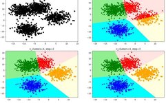
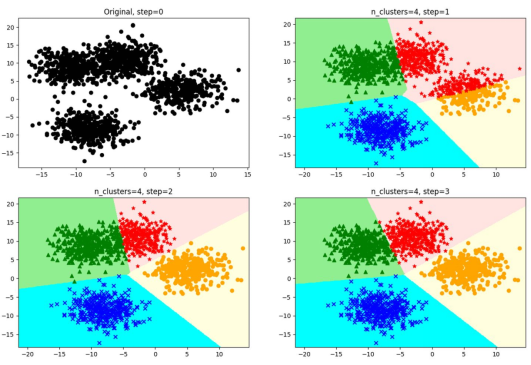
e. When the centroids do not change (when we find a centroid, and the samples assigned to this centroid remain consistent in each iteration, meaning that the newly generated clusters remain consistent and no sample points transfer from one cluster to another, the centroids will not change), stop and output the clustering results. The computation process of the K-Means algorithm is shown in Figure 1:
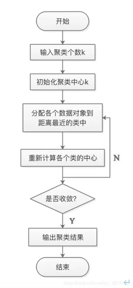
Figure 1 K-Means Algorithm Computation Process
Figure 2 K-Means Iteration Schematic
1. For the following data points, please use the K-Means method for clustering (manual calculation). Assume the number of clusters k=3, and the initial cluster centers are data point 2, data point 3, and data point 5.
Starting the first iteration with initial centroids B, C, E
AB = 2.502785
AC = 5.830635
AE = 7.054443
DB = 3.819911
DC = 1.071534
DE = 7.997158
Thus, the first cluster: {A, B}; the second cluster: {C, D}; the third cluster: {E}
That is, [array([-5.379713, -3.362104]), array([-3.487105, -1.724432])]
[array([ 0.450614, -3.302219]), array([-0.39237, -3.963704])]
[array([-3.45368, 3.424321])]
So the centroid of the first cluster is F: [-4.433409 -2.543268]
The centroid of the second cluster is G: [ 0.029122 -3.6329615]
The centroid of the third cluster is H: [-3.45368 3.424321]
###########################################################
Starting the second iteration
AF = 1.251393
AG = 5.415613
AH = 7.054443
BF = 1.251393
BG = 4.000792
BH = 5.148861
CF = 4.942640
CG = 0.535767
CH = 7.777522
DF = 4.283414
DG = 0.535767
DH = 7.997158
EF = 6.047478
EG = 7.869889
EH = 0.000000
Thus, the first cluster: {A, B}; the second cluster: {C, D}; the third cluster: {E}
That is, [array([-5.379713, -3.362104]), array([-3.487105, -1.724432])]
[array([ 0.450614, -3.302219]), array([-0.39237, -3.963704])]
[array([-3.45368, 3.424321])]
So the centroid of the first cluster is: [-4.433409 -2.543268]
The centroid of the second cluster is: [ 0.029122 -3.6329615]
The centroid of the third cluster is: [-3.45368 3.424321]
###########################################################
Since the members of the three clusters remain unchanged, the clustering ends
In summary: the first cluster: {A, B}; the second cluster: {C, D}; the third cluster: {E}
2. Definition of Intra-Cluster Sum of Squares
What do the classes obtained from the clustering algorithm signify? What properties do these classes possess?
We believe that data points within the same cluster have similarities, while data from different clusters are distinct. After clustering is completed, we need to study the properties of the samples in each cluster to formulate different business or technological strategies based on business needs. Clustering algorithms pursue “small intra-cluster variance and large inter-cluster variance.” This “variance” is measured by the distance of sample points to their cluster centroids.
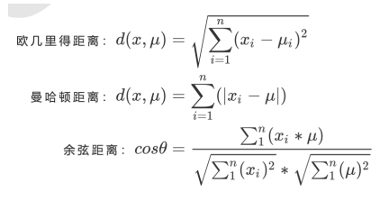
For a cluster, the smaller the sum of distances of all sample points to the centroid, the more similar the samples within that cluster are, and the smaller the intra-cluster variance. There are various methods to measure distance, letting x represent a sample point in the cluster, μ represent the centroid of that cluster, n represent the number of features in each sample point, and i represent each feature that makes up point x, then the distance of the sample point to the centroid can be measured by the following distance:
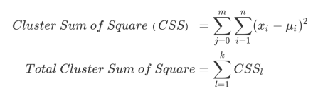
If using Euclidean distance, the sum of squared distances of all sample points in a cluster to the centroid is:
Where m is the number of samples in a cluster, and j is the sample number. This formula is called the Intra-Cluster Sum of Squares (Cluster Sum of Square), also known as Inertia. By summing the intra-cluster sum of squares of all clusters in a dataset, we obtain the Total Cluster Sum of Squares, also known as Total Inertia. The smaller the Total Inertia, the more similar the samples within each cluster, indicating better clustering results. Therefore, K-Means aims to find centroids that minimize Inertia. In fact, during the iterative process of changing centroids, the overall sum of squares decreases. We can mathematically prove that when the overall sum of squares reaches its minimum value, the centroids will no longer change. Thus, the K-Means solution process becomes an optimization problem.
In K-Means, under a fixed number of clusters K, the optimal centroids are solved by minimizing the overall sum of squares, and clustering is performed based on the existence of these centroids. The two processes are quite similar, and the minimum value of the overall distance squared can actually be solved using gradient descent.
It can be observed that Inertia is derived from the calculation formula based on Euclidean distance. In fact, other distances can also be used, each with its corresponding Inertia. From past experiences, different centroid selection methods and Inertia corresponding to different distances have been summarized. In K-Means, as long as the correct centroid and distance combination is used, good clustering results can be achieved regardless of the distance used.
|
|
|
|
|
|
|
Minimize the sum of Euclidean distances from each sample point to the centroid
|
|
|
|
Minimize the sum of Manhattan distances from each sample point to the centroid
|
|
|
|
Minimize the sum of cosine distances from each sample point to the centroid
|
3. Time Complexity of K-Means Algorithm
It is well known that algorithm complexity is divided into time complexity and space complexity. Time complexity refers to the amount of computational work required to execute an algorithm, commonly expressed in Big O notation; while space complexity refers to the amount of memory space required to execute the algorithm. If an algorithm performs well but has high time and space complexity, there will be a trade-off between the algorithm’s performance and the computational cost required.
The average complexity of the K-Means algorithm is O(k*n*T), where k is the hyperparameter, i.e., the number of clusters to be input, n is the number of samples in the entire dataset, and T is the number of iterations required. In the worst case, the complexity of K-Means can be expressed as O(n(k+2)/p), where n is the number of samples in the entire dataset, and p is the total number of features.
4. Model Evaluation Metrics for Clustering Algorithms
Unlike classification models and regression, evaluating clustering algorithms is not a simple task. In classification, there is a direct output of results (labels), and the results can be classified as correct or incorrect, so evaluation is done using metrics like prediction accuracy, confusion matrix, ROC curve, etc. However, no matter how evaluated, it is assessing “the model’s ability to find the correct answer.” In regression, since the model needs to fit the data, metrics like SSE mean squared error and loss function are used to measure the model’s fit. However, these metrics cannot be used for clustering.
The results of clustering models do not output a certain label, and the results of clustering are uncertain; their quality is determined by business needs or algorithm requirements, and there are no eternally correct answers. So how can we measure the effectiveness of clustering?
The goal of K-Means is to ensure “small intra-cluster variance and large inter-cluster variance,” so we can measure clustering effectiveness by assessing intra-cluster variance. As mentioned earlier, Inertia is an indicator used to measure intra-cluster variance, so can we use Inertia as a measure of clustering effectiveness?
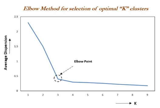
The “Elbow Method” suggests that the inflection point in Figure 3 is the optimal value of k.
The core idea of the Elbow Method: As the number of clusters k increases, the sample division becomes more refined, and the aggregation degree of each cluster gradually increases, thus Inertia will naturally decrease. When k is less than the actual number of clusters, the increase in k will significantly enhance the aggregation degree of each cluster, leading to a substantial decrease in Inertia. However, when k reaches the actual number of clusters, further increasing k will result in diminishing returns in aggregation degree, causing the decrease in Inertia to slow down and eventually become stable. This means that the relationship graph of Inertia and k resembles an elbow shape, and the k value at this elbow corresponds to the true number of clusters in the data. For example, in the figure below, the elbow corresponds to k=3 (highest curvature), indicating that the optimal number of clusters for this dataset should be set to 3.
 This raises a question: Is a smaller Inertia better for the model? The answer is that it can be, but the Inertia metric has its drawbacks and limitations:
a. Its calculation is too susceptible to the number of features.
b. It is unbounded; while smaller Inertia is better, it is unclear when the model has reached its limit and whether it can continue to improve.
c. It is influenced by the hyperparameter K; as K increases, Inertia will inevitably decrease, but this does not mean the model’s performance is improving.
d. Inertia assumes a certain distribution of data; it presumes that the data follows a convex distribution and is isotropic, thus using Inertia as an evaluation metric can lead to poor performance of clustering algorithms on elongated clusters, ring-shaped clusters, or irregularly shaped manifolds.
What other metrics can be used to evaluate model performance?
(1) Silhouette Coefficient
In 99% of cases, clustering is performed on data without true labels, that is, clustering on data where the true answers are unknown. Such clustering relies entirely on evaluating the density of samples within clusters (small intra-cluster variance) and the dispersion of samples between clusters (large inter-cluster variance) to assess clustering effectiveness. Among these, the silhouette coefficient is the most commonly used metric for clustering algorithms. It is defined for each sample and can simultaneously measure:
a) The similarity of a sample to other samples in its own cluster a, which equals the average distance between the sample and all other points in the same cluster.
b) The similarity of the sample to samples in other clusters b, which equals the average distance between the sample and all points in the nearest cluster.
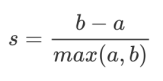
Based on the principle of clustering “small intra-cluster variance and large inter-cluster variance,” we hope that b is always greater than a, and the greater the difference, the better. The silhouette coefficient for a single sample is calculated as:
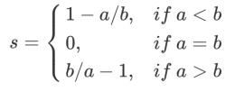
The formula can be expanded as:
It is easy to understand that the range of the silhouette coefficient is (-1,1), where a value closer to 1 indicates that the sample is very similar to other samples in its cluster and dissimilar to samples in other clusters. When a sample point is more similar to samples outside its cluster, the silhouette coefficient will be negative. When the silhouette coefficient is 0, it indicates that the samples in the two clusters are equally similar, suggesting that the two clusters should be merged into one.
If most samples in a cluster have a relatively high silhouette coefficient, the cluster will have a high total silhouette coefficient; thus, the average silhouette coefficient of the entire dataset indicates that the clustering is appropriate. Conversely, if many sample points have low silhouette coefficients or even negative values, the clustering is inappropriate, and the hyperparameter K may be set too high or too low.
The silhouette coefficient has many advantages; it takes values in a limited space, providing a “reference” for model clustering effectiveness. Moreover, the silhouette coefficient has no restrictions on data distribution, thus performing well on many datasets. It performs best when the segmentation of each cluster is relatively clear. However, the silhouette coefficient also has drawbacks; it tends to overestimate performance on convex clusters, such as those obtained through density-based clustering or clustering results obtained via DBSCAN, if evaluated using the silhouette coefficient, it may yield a score that is higher than the actual clustering effectiveness.
(2) Calinski-Harabasz Index
In addition to the silhouette coefficient, there are other metrics such as the Calinski-Harabasz Index (CHI), also known as the Variance Ratio Criterion, Davies-Bouldin Index, and Contingency Matrix. These will not be elaborated here; interested readers can study them independently.
5. The Issue of Initial Centroids
In K-Means, an important step is placing the initial centroids. If there is enough time, K-Means will definitely converge, but Inertia may converge to a local minimum. Whether it can converge to the true minimum value largely depends on the initialization of the centroids.
The placement of initial centroids can significantly affect clustering results; a good choice of centroids can help K-Means avoid excessive computations, leading to stable and faster convergence. When discussing the placement of initial centroids earlier, a “random” method was used to select k samples from the sample points as initial centroids, which clearly does not meet the requirement for “stability and speed.”
To address this, the random_state parameter in sklearn can be used to control and ensure that the initial centroids generated each time are at the same position; learning curves can also be drawn to determine the optimal random_state parameter.
A random_state corresponds to a random seed for initializing centroids. If no random seed is specified, K-Means in sklearn will not select a single random mode to produce results but will run multiple times under each random seed and use the best result as the initial centroid.
In sklearn, the n_init parameter can also be used to select the number of runs under each random seed, and increasing this n_init value can enhance the number of runs under each random seed.
Additionally, to optimize the method of selecting initial centroids, “k-means++” can be used to ensure that initial centroids are spaced apart, leading to more reliable results than random initialization. In sklearn, the parameter init=’k-means++’ can be used to choose k-means++ as the centroid initialization scheme.
6. Iteration Issues in Clustering Algorithms
As we all know, when the centroids stop moving, the K-Means algorithm will stop. Before complete convergence, parameters max_iter (maximum number of iterations) or tol can also be used in sklearn to allow for early stopping of iterations. Sometimes, when n_clusters is not aligned with the natural distribution of the data, or for business needs, forcing the input of n_clusters can enhance the model’s performance by stopping iterations early.
max_iter: integer, default 300, the maximum number of iterations for a single run of the K-Means algorithm;
tol: float, default 1e-4, the amount of decrease in Inertia between two iterations; if the decrease is less than the set tol value, the iteration will stop.
7. Advantages and Disadvantages of K-Means Algorithm
(1) Advantages of K-Means Algorithm
This raises a question: Is a smaller Inertia better for the model? The answer is that it can be, but the Inertia metric has its drawbacks and limitations:
a. Its calculation is too susceptible to the number of features.
b. It is unbounded; while smaller Inertia is better, it is unclear when the model has reached its limit and whether it can continue to improve.
c. It is influenced by the hyperparameter K; as K increases, Inertia will inevitably decrease, but this does not mean the model’s performance is improving.
d. Inertia assumes a certain distribution of data; it presumes that the data follows a convex distribution and is isotropic, thus using Inertia as an evaluation metric can lead to poor performance of clustering algorithms on elongated clusters, ring-shaped clusters, or irregularly shaped manifolds.
What other metrics can be used to evaluate model performance?
(1) Silhouette Coefficient
In 99% of cases, clustering is performed on data without true labels, that is, clustering on data where the true answers are unknown. Such clustering relies entirely on evaluating the density of samples within clusters (small intra-cluster variance) and the dispersion of samples between clusters (large inter-cluster variance) to assess clustering effectiveness. Among these, the silhouette coefficient is the most commonly used metric for clustering algorithms. It is defined for each sample and can simultaneously measure:
a) The similarity of a sample to other samples in its own cluster a, which equals the average distance between the sample and all other points in the same cluster.
b) The similarity of the sample to samples in other clusters b, which equals the average distance between the sample and all points in the nearest cluster.
Based on the principle of clustering “small intra-cluster variance and large inter-cluster variance,” we hope that b is always greater than a, and the greater the difference, the better. The silhouette coefficient for a single sample is calculated as:
The formula can be expanded as:
It is easy to understand that the range of the silhouette coefficient is (-1,1), where a value closer to 1 indicates that the sample is very similar to other samples in its cluster and dissimilar to samples in other clusters. When a sample point is more similar to samples outside its cluster, the silhouette coefficient will be negative. When the silhouette coefficient is 0, it indicates that the samples in the two clusters are equally similar, suggesting that the two clusters should be merged into one.
If most samples in a cluster have a relatively high silhouette coefficient, the cluster will have a high total silhouette coefficient; thus, the average silhouette coefficient of the entire dataset indicates that the clustering is appropriate. Conversely, if many sample points have low silhouette coefficients or even negative values, the clustering is inappropriate, and the hyperparameter K may be set too high or too low.
The silhouette coefficient has many advantages; it takes values in a limited space, providing a “reference” for model clustering effectiveness. Moreover, the silhouette coefficient has no restrictions on data distribution, thus performing well on many datasets. It performs best when the segmentation of each cluster is relatively clear. However, the silhouette coefficient also has drawbacks; it tends to overestimate performance on convex clusters, such as those obtained through density-based clustering or clustering results obtained via DBSCAN, if evaluated using the silhouette coefficient, it may yield a score that is higher than the actual clustering effectiveness.
(2) Calinski-Harabasz Index
In addition to the silhouette coefficient, there are other metrics such as the Calinski-Harabasz Index (CHI), also known as the Variance Ratio Criterion, Davies-Bouldin Index, and Contingency Matrix. These will not be elaborated here; interested readers can study them independently.
5. The Issue of Initial Centroids
In K-Means, an important step is placing the initial centroids. If there is enough time, K-Means will definitely converge, but Inertia may converge to a local minimum. Whether it can converge to the true minimum value largely depends on the initialization of the centroids.
The placement of initial centroids can significantly affect clustering results; a good choice of centroids can help K-Means avoid excessive computations, leading to stable and faster convergence. When discussing the placement of initial centroids earlier, a “random” method was used to select k samples from the sample points as initial centroids, which clearly does not meet the requirement for “stability and speed.”
To address this, the random_state parameter in sklearn can be used to control and ensure that the initial centroids generated each time are at the same position; learning curves can also be drawn to determine the optimal random_state parameter.
A random_state corresponds to a random seed for initializing centroids. If no random seed is specified, K-Means in sklearn will not select a single random mode to produce results but will run multiple times under each random seed and use the best result as the initial centroid.
In sklearn, the n_init parameter can also be used to select the number of runs under each random seed, and increasing this n_init value can enhance the number of runs under each random seed.
Additionally, to optimize the method of selecting initial centroids, “k-means++” can be used to ensure that initial centroids are spaced apart, leading to more reliable results than random initialization. In sklearn, the parameter init=’k-means++’ can be used to choose k-means++ as the centroid initialization scheme.
6. Iteration Issues in Clustering Algorithms
As we all know, when the centroids stop moving, the K-Means algorithm will stop. Before complete convergence, parameters max_iter (maximum number of iterations) or tol can also be used in sklearn to allow for early stopping of iterations. Sometimes, when n_clusters is not aligned with the natural distribution of the data, or for business needs, forcing the input of n_clusters can enhance the model’s performance by stopping iterations early.
max_iter: integer, default 300, the maximum number of iterations for a single run of the K-Means algorithm;
tol: float, default 1e-4, the amount of decrease in Inertia between two iterations; if the decrease is less than the set tol value, the iteration will stop.
7. Advantages and Disadvantages of K-Means Algorithm
(1) Advantages of K-Means Algorithm
-
The principle is relatively simple, and implementation is easy, with fast convergence speed;
-
Clustering effects are relatively good, and the algorithm has strong interpretability.
(2) Disadvantages of K-Means Algorithm
-
The selection of K value is difficult to grasp;
-
It is challenging to converge for non-convex datasets;
-
If the data of each hidden category is imbalanced, such as severe imbalance in data volume or different variances among categories, clustering performance may be poor;
-
Using iterative methods, the results obtained are only locally optimal;
-
It is sensitive to noise and outliers.
The K-Means clustering algorithm has a simple principle, strong interpretability, and convenient implementation, making it widely applicable in various fields such as data mining, clustering analysis, data clustering, pattern recognition, financial risk control, data science, intelligent marketing, and data operations, with broad application prospects.
Introduction to DataPi Research Department
The DataPi Research Department was established in early 2017, dividing into multiple groups based on interest, each group follows the overall knowledge sharing and practical project planning of the research department while having its unique characteristics:
Algorithm Model Group: Actively participates in competitions like Kaggle, original hands-on tutorial series;
Research and Analysis Group: Conducts research on the application of big data through interviews, exploring the beauty of data products;
System Platform Group: Tracks cutting-edge technologies in big data & artificial intelligence system platforms and dialogues with experts;
Natural Language Processing Group: Focuses on practice, actively participates in competitions and plans various text analysis projects;
Manufacturing Big Data Group: Upholds the dream of being a strong industrial nation, combining industry, academia, research, and government to uncover data value;
Data Visualization Group: Merges information with art, explores the beauty of data, and learns to tell stories through visualization;
Web Crawler Group: Crawls web information and collaborates with other groups to develop creative projects.
Click on the end of the article “Read the original text” to sign up for DataPi Research Department volunteers, there is always a group that suits you~
Reprint Notice
If you need to reprint, please prominently indicate the author and source at the beginning (originally from: DataPi THUID: DatapiTHU), and place a prominent QR code of DataPi at the end of the article. For articles with original identification, please send 【article name -待授权公众号名称及ID】 to the contact email to apply for whitelist authorization and edit as required.
Unauthorized reprints and adaptations will be legally pursued.
Click “Read the original text” to join the organization~