Understanding Gradient Descent in Neural Networks

This article will coverthe essence of Gradient Descent, the principles of Gradient Descentand the algorithms of Gradient Descent in three aspects, helping you understand Gradient Descent Gradient Descent | GD.

Gradient Descent

1.Essence of Gradient Descent

Machine Learning’s “Three Essentials”: Select a model family, define a loss function to quantify prediction errors, and find the optimal model parameters that minimize the loss using optimization algorithms.

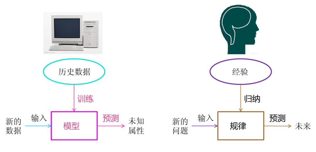
Machine Learning vs Human Learning

• Define a set of functions (model selection)

• Goal: Determine an appropriate hypothesis space or model family.

• Example: Linear Regression, Logistic Regression, Neural Networks, Decision Trees, etc.

• Considerations: Complexity of the problem, nature of the data, computational resources, etc.

• Evaluate the quality of functions (loss function)

• Goal: Quantify the difference between model predictions and actual results.

• Example: Mean Squared Error (MSE) for regression; Cross-entropy loss for classification.

• Considerations: Nature of the loss (convexity, differentiability, etc.), ease of optimization, robustness to outliers, etc.

• Select the best function (optimization algorithm)

• Goal: Find model parameters that minimize the loss function within the set of functions.

• Main methods: Gradient Descent and its variants (Stochastic Gradient Descent, Mini-batch Gradient Descent, Adam, etc.).

• Considerations: Convergence speed, computational efficiency, complexity of parameter tuning, etc.

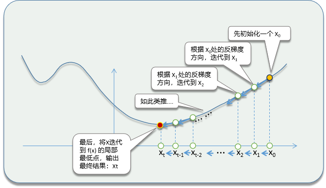
Essence of Gradient Descent:Used to solve optimization problems in machine learning and deep learning.

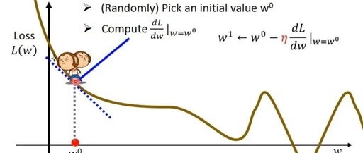
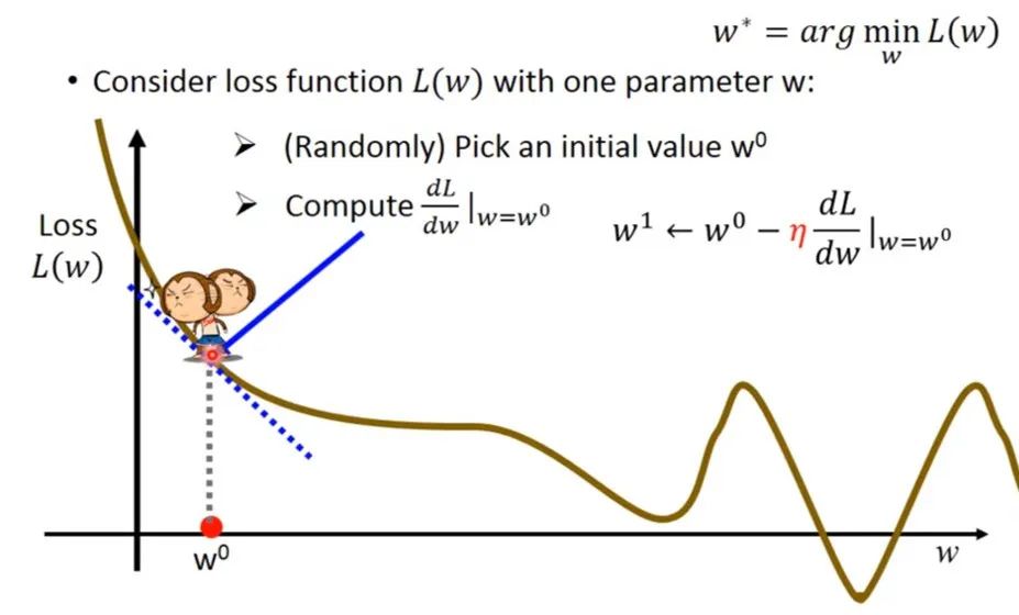
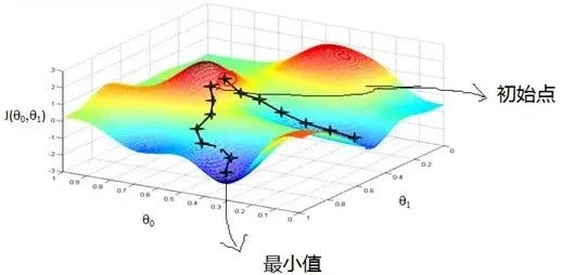
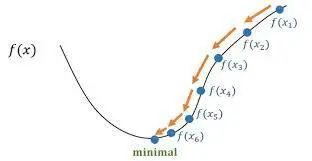
The basic idea of Gradient Descent is to start from an initial point and continuously update parameters in the direction of the negative gradient of the loss function until reaching a local minimum or global minimum.

Basic idea of Gradient Descent

• Initialize parameters: Choose an initial parameter value.

• Calculate the gradient: Compute the gradient of the loss function at the current parameter value.

• Update parameters: Update parameters in the opposite direction of the gradient, usually using a learning rate to control the step size.

• Repeat iterations: Repeat steps 2 and 3 until the stopping condition is met (e.g., maximum iterations reached, loss function value below a threshold, etc.).

Key steps of Gradient Descent

2.Principles of Gradient Descent

In Gradient Descent, the minimum of the directional derivative (i.e., the opposite direction of the gradient) is used to update parameters, thereby approaching the minimum of the function.

Directional Derivative: In the Gradient Descent algorithm, the directional derivative is used to determine the fastest direction for the function value to decrease.

• Definition: The directional derivative is the rate of change of a function at a specific point in a specific direction. For multivariable functions, it represents the instantaneous rate of change of the function value in a certain direction at that point.

• Properties: The magnitude of the directional derivative depends on the gradient of the function at that point and the choice of the direction vector. When the direction vector aligns with the gradient direction, the directional derivative reaches its maximum; when the direction vector is opposite to the gradient direction, the directional derivative reaches its minimum.

• Relationship with Gradient Descent: In the Gradient Descent algorithm, the directional derivative is used to determine the fastest direction for the function value to decrease. By calculating the directional derivative in the negative gradient direction, we can find the direction that decreases the function value, thereby updating parameters to approach the minimum of the function.

Directional Derivative

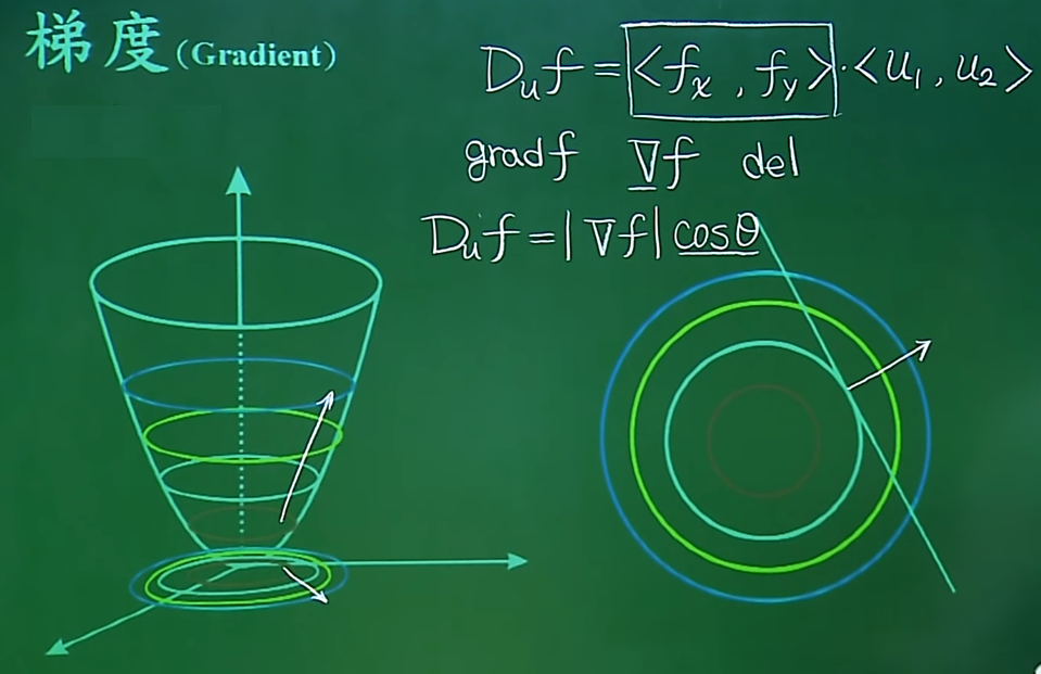
Gradient (Gradient):In the Gradient Descent algorithm, the gradientprovides information about the direction and rate of decrease of the function.

• Definition: The gradient is a vector whose components are the partial derivatives of the function with respect to the corresponding variables. For multivariable functions, the gradient represents the maximum rate of change of the function at a point and the direction of that change.

• Properties: The direction of the gradient always points towards the direction of the fastest increase of the function value, while the magnitude (length) of the gradient indicates the maximum rate of change in that direction. At the stationary points of the function (where the gradient is zero), the function may reach a local minimum, local maximum, or saddle point.

• Relationship with Gradient Descent: The Gradient Descent algorithm uses the gradient information to update parameters to minimize the objective function. In each iteration, the algorithm calculates the gradient at the current point and moves a certain step length in the opposite direction of the gradient (negative gradient direction), which is typically controlled by the learning rate.

Gradient

3. Gradient Descent Algorithm

Batch Gradient Descent (BGD): In each iteration, Batch Gradient Descent uses the entire dataset to calculate the gradient of the loss function and updates all model parameters based on this gradient.

Batch Gradient Descent (BGD)

• Advantages:

  Stable convergence: Because it uses the entire dataset to calculate the gradient, Batch Gradient Descent usually converges more stably to the minimum of the loss function, avoiding drastic fluctuations during the optimization process.

  Global perspective: It considers all samples in the dataset for parameter updates, which helps the model gain a global perspective rather than just focusing on a single sample or a small subset of samples.

  Easy to implement: The Batch Gradient Descent algorithm is relatively simple and easy to understand and implement.

• Disadvantages:

  High computational cost: When the dataset is very large, the computational cost of Batch Gradient Descent can become very high, as each iteration requires processing the entire dataset.

  High memory consumption: Since the entire dataset needs to be loaded into memory at once, Batch Gradient Descent has relatively high memory requirements.

  Slow update speed: Since each update is based on the average gradient of the entire dataset, Batch Gradient Descent may update parameters more slowly than Stochastic Gradient Descent in some cases.

Stochastic Gradient Descent (SGD)::Unlike Batch Gradient Descent, Stochastic Gradient Descent randomly selects one sample in each iteration to calculate the gradient of the loss function and updates one or more model parameters based on this gradient.

Stochastic Gradient Descent (SGD)

Advantages:

1. High computational efficiency: Since each iteration only processes one sample, the computational efficiency of Stochastic Gradient Descent is usually much higher than that of Batch Gradient Descent, especially when dealing with large datasets.

2. Low memory consumption: Stochastic Gradient Descent only needs to load one sample into memory at a time, so its memory requirements are relatively low.

3. Helps escape local minima: Because each update is based on the gradient of a single sample, Stochastic Gradient Descent has greater randomness in the optimization process, which helps the model escape local minima and find better global minima.

Disadvantages:

1. Unstable convergence process: Since each update is based on the gradient of a single sample, the convergence process of Stochastic Gradient Descent is usually less stable than that of Batch Gradient Descent, which may result in larger fluctuations.

2. Difficult to reach global optimum: In some cases, Stochastic Gradient Descent may get stuck in local minima and fail to reach the global optimum.

3. Requires additional techniques: To improve the performance and stability of Stochastic Gradient Descent, additional techniques such as gradually decreasing the learning rate (learning rate decay), using momentum, etc., are often required.