
Source: PaperWeekly
Source
This article is a compilation of some technical blogs and overviews that I recently read about diffusion models, mainly referencing Calvin Luo’s paper, aimed at readers who already have some basic understanding of diffusion models.
Calvin Luo’s paper provides a unified perspective for understanding diffusion models, especially with detailed mathematical derivations. This article will attempt to briefly summarize the derivation process of diffusion models from a unified perspective. At the end, I will include some thoughts and questions regarding the strong assumptions made during the derivation process, and briefly discuss some considerations when applying diffusion models in natural language processing.
This reading note references the following technical blogs. Readers unfamiliar with diffusion models may consider first reading Lilian Weng’s popular science blog. Calvin Luo’s introductory paper has been reviewed by several authors of related diffusion model papers, including Jonathan Ho (author of DDPM), Dr. Song Yang, and others, making it highly recommended.
1. What are Diffusion Models? by Lilian Weng:
https://lilianweng.github.io/posts/2021-07-11-diffusion-models/
2. Generative Modeling by Estimating Gradients of the Data Distribution by Song Yang:
https://yang-song.net/blog/2021/score/
3. Understanding Diffusion Models: A Unified Perspective by Calvin Luo:
https://arxiv.org/abs/2208.11970
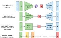
Generative models aim to generate data that conforms to the real distribution (or given dataset). Some common generative models include GANs, Flow-based Models, VAEs, Energy-Based Models, and the diffusion models we hope to discuss today. The diffusion models have some connections and differences with Variational Autoencoders (VAEs) and Energy-Based Models (EBMs), which I will elaborate on in the following sections.

▲ Common Generative Models
1. ELBO & VAE
Before introducing diffusion models, let’s first review Variational Autoencoders (VAEs). We know that the most significant feature of VAEs is the introduction of a latent vector distribution to assist in modeling the real data distribution.
So why do we introduce latent vectors? There are two intuitive reasons: one is that directly modeling high-dimensional representations is extremely difficult, often requiring strong prior assumptions and facing dimensionality organization issues. The other is that learning low-dimensional latent vectors directly serves both to compress dimensions and to explore semantic structural information in low-dimensional space (for example, in the image domain, GANs can often manipulate specific dimensions to influence particular features of the output image).
After introducing latent vectors, we can express the log-likelihood of our target distribution logP(x), also known as the “evidence,” in the following form:
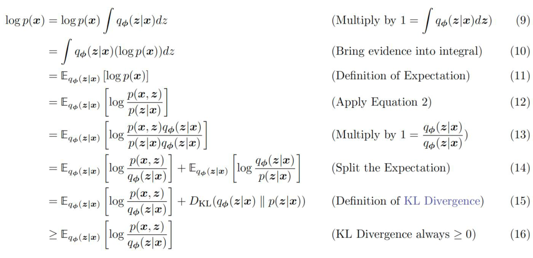
▲ ELBO Derivation Process
Here, we focus on equation 15. The left side of the equation is the real data distribution (evidence) that the generative model aims to approach, while the right side consists of two terms, where the second term’s KL divergence is always greater than zero, so the inequality holds. If we subtract this KL divergence from the right side of the equation, we obtain the lower bound of the real data distribution, known as the Evidence Lower Bound (ELBO). By further expanding ELBO, we can derive the optimization objective of VAE.
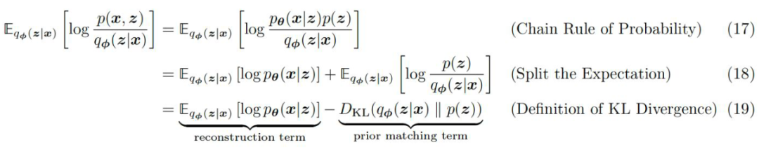
▲ Expansion of ELBO Equation
We can intuitively understand the form of this evidence lower bound: it is equivalent to a process where we encode the input x into a posterior latent vector distribution q(z|x) using an encoder. We hope this vector distribution closely resembles the true latent vector distribution p(z), so we constrain it using KL divergence, which also prevents the learned posterior distribution q(z|x) from collapsing into a Dirac delta function (the right side of equation 19). The obtained latent vector is then used by a decoder to reconstruct the original data, corresponding to the left side of equation 19 P(x|z).
Why is it called a Variational Autoencoder? The “variational” part comes from the process of finding the optimal latent vector distribution q(z|x). The “autoencoder” part refers to the aforementioned encoding of input data and the subsequent decoding back to the original data.
So to summarize why VAEs can fit the original data distribution well: based on the formula derivation mentioned above, we find that the log-likelihood of the original data distribution (referred to as evidence) can be expressed as the evidence lower bound plus the KL divergence between the posterior latent vector distribution we wish to approximate and the true latent vector distribution (i.e., equation 15). If we write this as A=B+C, we see that since evidence (A) is a constant (unrelated to the parameters we want to learn), maximizing B, which is our evidence lower bound, is equivalent to minimizing C, which is the difference between the distribution we want to fit and the true distribution. Because of the evidence lower bound, we can rewrite it in the form of an autoencoder, obtaining the training objective of the autoencoder. Optimizing this objective is equivalent to approximating the true data distribution, which is also equivalent to optimizing the posterior latent vector distribution q(z|x) using variational methods.
However, VAEs still have many issues. One of the most obvious is how we choose the posterior distribution. In most VAE implementations, this posterior distribution is chosen as a multi-dimensional Gaussian distribution. But this choice is more for computational and optimization convenience. Such a simple form greatly limits the model’s ability to approximate the true posterior distribution. The original authors of VAE, Kingma, had a very classic work that improved the expressiveness of the posterior distribution by introducing normalization flow [1]. Diffusion models can also be seen as an improvement to the posterior distribution.
2. Hierarchical VAE
The following diagram shows the closed-loop relationship between the latent vector and the input in a variational autoencoder. That is, after extracting the low-dimensional latent vector from the input, we can reconstruct the input using this latent vector.
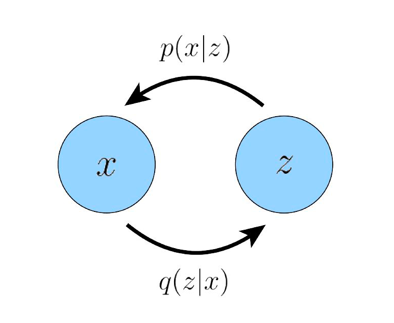
▲ Relationship between Latent Vector and Input in VAE
It is clear that we believe this low-dimensional latent vector must efficiently encode some important characteristics of the original data distribution, allowing our decoder to successfully reconstruct various data from the original data distribution. So if we recursively calculate the “latent vector of the latent vector,” we obtain a multi-layer Hierarchical Variational Autoencoder (HVAE), where each layer’s latent vector is conditioned on all preceding latent vectors.
However, in this article, we mainly focus on the Markovian Hierarchical Variational Autoencoder (MHVAE), where each layer’s latent vector is only conditioned on the previous layer’s latent vector.
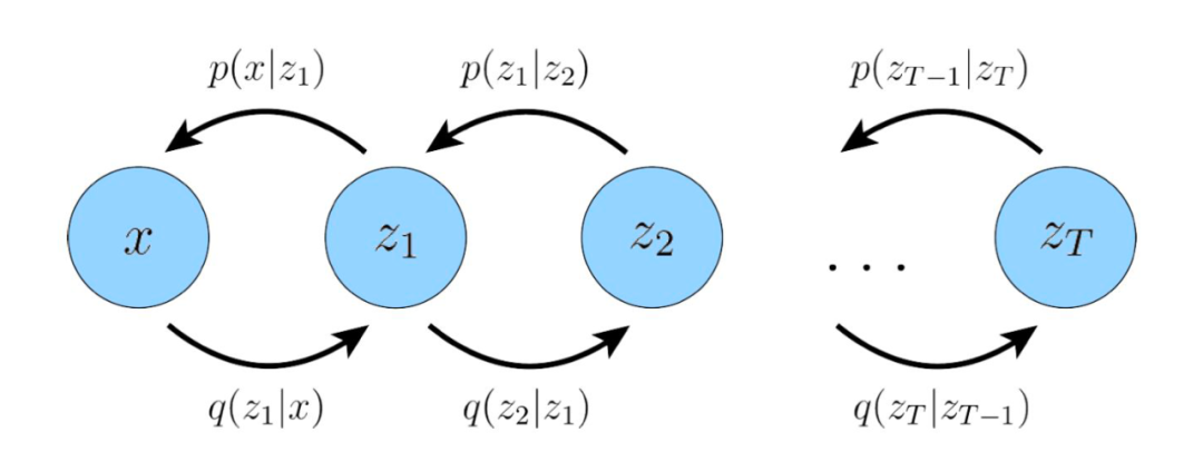
▲ In MHVAE, the latent vector is conditioned only on the previous layer
For this MHVAE, we can derive the evidence lower bound through the following steps:
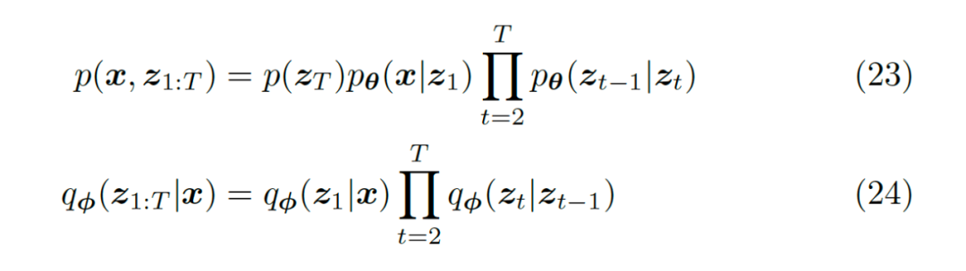
▲ Derivation of the Variational Lower Bound for MHVAE
3. Variation Diffusion Model
The reason we spent so much space introducing VAE and deriving the evidence lower bound for MHVAE before discussing diffusion models is that we can naturally view diffusion models as a special case of MHVAE, which satisfies the following three constraints (note that these three constraints are also the foundation of the entire diffusion model inference):
-
The dimension of the latent vector Z is consistent with the dimension of the input X.
-
Each time step’s latent vector is encoded as a Gaussian distribution that only depends on the previous time step’s latent vector.
-
The parameters of the Gaussian distribution of each time step’s latent vector vary with the time step and satisfy the constraint that the Gaussian distribution at the final time step approaches the standard Gaussian distribution.
Due to the first point regarding dimensional consistency, without affecting understanding, we will represent Zt in MHVAE as Xt (where x0 is the original input), allowing us to redraw the dependency graph of the hierarchical latent vectors in MHVAE as follows (i.e., treating the intermediate diffusion process of the diffusion model as a hierarchical modeling process of latent vectors):
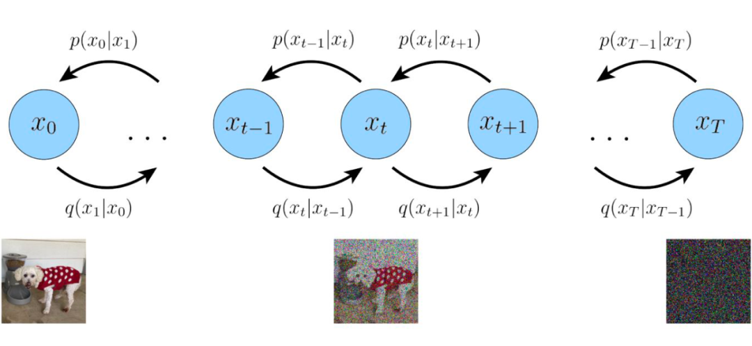
▲ Intuitive Explanation of the Diffusion Process: Continuously adding Gaussian noise to data x0 until it degrades into pure noise image Xt
At this point, we finally see the familiar form of diffusion models.
By replacing Zt with Xt in the above equations 25-28, we can obtain the first four lines of the derivation formula for the evidence lower bound in VDM, i.e., equations 34-37. Furthermore, we can continue to derive further.
The transformation from line 37 to 38 is an equivalent substitution based on the chain rule (or the transformations in the above equations 23 and 24), while the transformation from line 38 to 39 is a reorganization of the multiplication process, from 39 to 40 aligns the multiplication symbols, from 40 to 41 applies the properties of logarithmic multiplication, and from 41 to 42 further splits using the same property, from 42 to 43 is because the expectation of a sum equals the sum of expectations, from 43 to 44 is because the expected target is independent of the probabilities of some time steps and can be directly omitted, and from 44 to 45 applies the definition of KL divergence for reorganization.
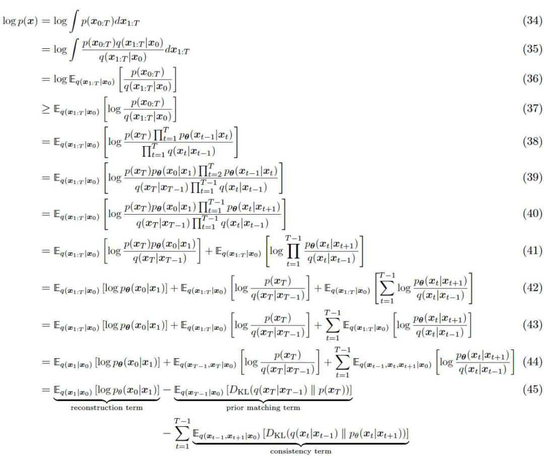
▲ Derivation of the Evidence Lower Bound for VDM
At this point, we once again transformed the log-likelihood of the original data distribution into the evidence lower bound (equation 37), and transformed it into a very intuitive form of a sum of several loss functions (equation 45), which are:
-
The reconstruction term, which changes from the latent vector to the original data. In VAE, this reconstruction term is written as , while here we write it as .
-
The prior matching term. Recall that we mentioned above that the final time step’s Gaussian distribution should be established as a standard Gaussian distribution.
-
The consistency term. This loss term is designed to ensure that the distribution of Xt during the forward noise-adding process remains consistent with the backward denoising process. Intuitively, the denoising of a more chaotic image should be consistent with the noise-adding of a clearer image. Since the consistency term’s loss is defined over all time steps, it is also the most time-consuming calculation among the three loss terms.
Although the above formula derivation gives us a very intuitive evidence lower bound, and since each term is calculated as an expectation, it is naturally suitable for Monte Carlo methods for approximation, several problems still exist in optimizing this evidence lower bound:
-
Our consistency term loss is an expectation based on two random variables. The variance of their Monte Carlo estimates is likely larger than the variance of Monte Carlo estimates based on a single independent variable.
-
Our consistency term is defined as the sum of KL divergence expectations over all time steps. In cases where T takes a high value (usually around 2000 for diffusion models), the variance of this expectation will also be large.
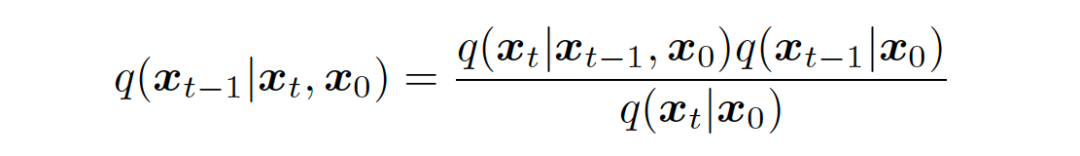
Thus, we need to derive a new evidence lower bound. The key to this derivation will focus on the following observation: we can rewrite the forward noise-adding process of the diffusion process as . The reason for this rewriting is based on the Markov assumption, where these two equations are entirely equivalent. Therefore, by applying Bayes’ theorem to this equation, we can obtain equation 46.
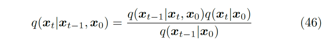
▲ Formula after applying the Markov assumption and Bayes’ theorem to the forward noise-adding process
Based on equation 46, we can rewrite the above evidence lower bound (equation 37) in the following form, where equations 47, 48, and equations 37, 38 are consistent. Starting from equation 49, the multiplication in the denominator is decomposed from T to 1. In equation 50, based on the previously mentioned Markov assumption, we add the dependence of to the denominator. Equation 51 splits the logarithmic target using the properties of logarithms.
Equation 52 substitutes equation 46 for replacement. In equation 53, we extract the canceled denominator part and find that the remaining terms can be reduced to part of equation 54. Equation 54 uses the properties of logarithms to eliminate . In equations 56, we apply the properties of KL divergence.
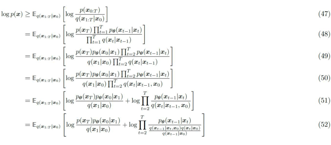
▲ Evidence Lower Bound Derivation for Diffusion Model after Applying the Markov Assumption
▲ Evidence Lower Bound Derivation for Diffusion Model after Applying the Markov Assumption 2
At this point, we have derived a better evidence lower bound by applying the Markov assumption. This evidence lower bound also includes several intuitive loss functions:
-
The reconstruction term. This reconstruction term is consistent with the one mentioned above.
-
The prior matching term. Slightly different from the one mentioned above, but still based on the assumption that the final time step should be a standard Gaussian.
- The denoising matching term. The most significant difference from the previously mentioned consistency term is that it is no longer an expectation based on two random variables. Intuitively, represents the backward denoising process, while represents the forward noise-adding process of the known original image and target noisy image. This noise-adding process serves as the target signal to supervise the backward denoising process. This term addresses the issue of expectations being based on two random variables.
Note that the above derivation is entirely based on the Markov property, so it applies to all MHVAE. Therefore, when T=1, the evidence lower bound obtained above is completely consistent with the evidence lower bound derived from VAE! Furthermore, the reason this article is called a unified perspective is that different papers have different optimization methods for the denoising matching term in this evidence lower bound. However, fundamentally, they are all equivalent in essence and can be derived from this expression.
Next, we will derive the formulas from the perspective of diffusion models to elaborate on calculating the denoising matching term. (Note that in the previous version of the derivation, the consistency term can also be obtained by deriving the expressions for q and p using the method in the next section, and then calculating the analytical form through KL.)
4. Diffusion Model Recap
In diffusion models, there are several important assumptions. One of them is that each transformation in the diffusion process is a Gaussian transformation of the previous step’s result (the second constraint of the previous section on MHVAE):
▲ Unlike MHVAE, the latent vector distribution on the encoder side is not learned, but is fixed as a linear Gaussian model
This is quite different from VAEs. In VAEs, the latent vector distribution on the encoder side is obtained through model training. In diffusion models, every step in the forward noise-adding process is based on the Gaussian transformation of the previous step’s result. The parameter is generally set as a hyperparameter. This greatly aids in calculating the evidence lower bound for diffusion models. Because we can know the exact state of a particular step in the forward process based on the input, we can supervise our predictions.
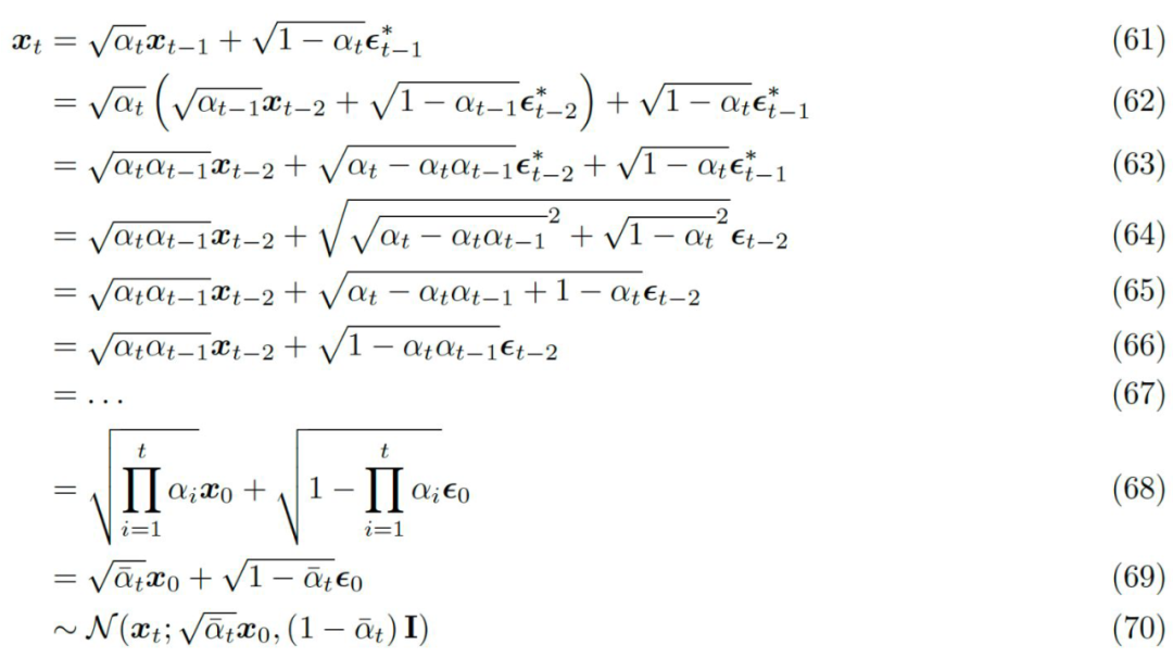
Based on equation 31, we can recursively add noise transformations to obtain the final expression for .

▲ can be expressed as a sampling result of a Gaussian distribution
Thus, for the supervision signal in the noise matching term of equation 58, we can rewrite it in the following form, where based on equation 70, we can obtain the expressions for and , and because it is the forward diffusion process, we can apply the Markov property to obtain specific expressions.
▲ The supervision signal in equation 58 can be computed for specific values
Substituting each term representing q into the Gaussian function expression, we ultimately obtain a new Gaussian distribution expression, where each term is computable:
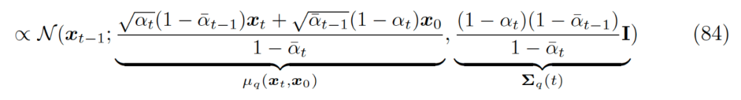
▲ The analytical form of
It has been proven that the forward noise-adding process can be expressed as a Gaussian distribution. In the initial paper on diffusion models [2], it was mentioned that for a continuous Gaussian diffusion process, its reverse process has the same equation form (functional form) as the forward process. Therefore, we will also adopt the Gaussian distribution form for the denoising matching term in this context (more specific derivations are provided in the appendix at the end). Note that in equation 58, the analytical solution form for the KL divergence between two Gaussian distributions is as follows:

Now that we know the parameters of one Gaussian distribution (the left side), if we set the variance of the Gaussian distribution on the right side to be consistent with that of the left side, then optimizing the analytical form of this KL divergence will simplify to the following form:
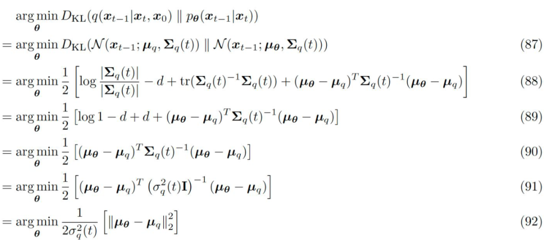
▲ The noise matching term in equation 58 is simplified to minimizing the prediction error of the forward and backward means
Thus, the noise matching term in equation 58 has been simplified to minimizing the prediction error of the forward and backward means (equation 92). Please note that the following three equivalent perspectives on the diffusion model essentially derive from different transformations of in equation 92. Here, is a function of , while is a function of and t. Through equation 84, we have the accurate calculation result of , while because is a function of .
We can express it in a form similar to equation 84(Note: The deeper reason behind why we can ignore variance and let the mean take this form is discussed in the appendix at the end. However, the choice of this form essentially opens up a new field of study, and research in this area directly led to the emergence of a series of accelerated sampling techniques following diffusion models).
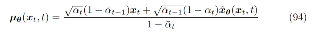
▲ Writing the backward predicted mean in a form similar to forward noise addition
Comparing equations 84 and 94, we see that is our neural network that predicts the original data from the noisy data . Therefore, we can finally express the noise matching term in the evidence lower bound of equation 58 as:
▲ The final form of the noise matching term
Thus, we have derived the optimization of diffusion models, ultimately expressed as training a neural network to predict the original image from any time step’s noisy image! At this point, the optimization objective has transformed into minimizing prediction errors. Meanwhile, the optimization of the noise matching terms summed over all time steps in equation 58 can be approximated as the minimum expected value of the prediction errors at each time step, and this optimization objective can be achieved through random sampling:

▲ This optimization objective can be achieved through random sampling
5. Three Equivalent Perspectives
Why is Calvin Luo’s paper titled Unified Perspective on diffusion models? We have spent a considerable amount of space demonstrating that the optimization objective of diffusion models can ultimately be transformed into training a neural network to predict the original input from any time step.
Next, we will discuss how to derive similar perspectives on diffusion models through different derivations.
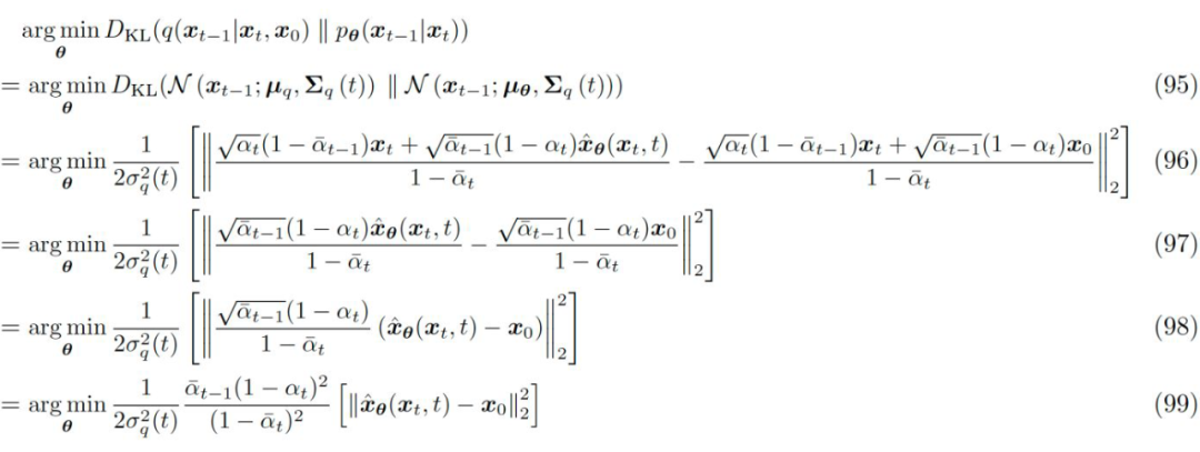
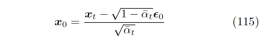
First, we already know that given the noise coefficient for each time step, we can recursively obtain from the initial input. Similarly, given , we can also derive . Therefore, resetting equation 69, we can obtain equation 115.

▲ Resetting the relationship between and in equation 69 gives us equation 115
By substituting equation 115 back into equation 84, we can derive the true mean expression regarding time step t.

▲ Deriving the true mean by substituting
Note that in the previous derivation process, the in was canceled out when calculating the analytical form of KL divergence, while was replaced with a neural network fitting strategy. In this derivation process, was replaced with an expression regarding (about and ), and we can obtain a new expression for that is still related to , just no longer related to (equation 124).
Where, like equation 94, we ignore the variance (setting it to be consistent with the forward process) and express the desired fitting of in a form similar to the true mean, only replacing with the fitting term of the neural network, yielding equation 125.

▲ Replacing with the neural network fitting term
Substituting the newly obtained two mean expressions back into the KL divergence expression, we find that they cancel out again (because the forms of and are consistent), leaving only the difference between and .Note the similarity between equations 130 and 99!
▲ The final optimization of the denoising matching term in the evidence lower bound can be expressed as the minimum of the difference between the initial noise and its fitting term
Thus, we have obtained the second intuitive understanding of diffusion models. For a Variational Diffusion Model (VDM), optimizing the evidence lower bound of this model is equivalent to optimizing the expected prediction error of the original image across all time steps, and it is also equivalent to optimizing the expected prediction error of the noise across all time steps! In fact, the approach taken by DDPM is precisely the method in equation 130 (note that the expression used in DDPM actually employs , which will also be discussed at the end).
Next, I will summarize the third way of viewing VDM. This approach mainly comes from Dr. Song Yang’s series of papers, which is very intuitive. Moreover, this series of papers unified the discrete multi-step denoising process of diffusion models into a special form of continuous stochastic differential equations (SDE). Dr. Song Yang thus won the Best Paper Award at ICLR 2021!
Subsequent papers from Tsinghua University, based on transforming this SDE into ordinary differential equations (ODE), also won the Best Paper Award at ICLR 2022! Dr. Song Yang provided very insightful and intuitive explanations of some details and understandings of this paper on his blog. Interested readers can check the second link at the beginning of this article. Below, I will briefly summarize the third perspective on the unified view.
The third derivation method is primarily based on Tweedie’s formula. This formula mainly describes that for a true mean of a distribution from an exponential family, given sampling samples, it can be estimated by the maximum likelihood probability of the sampling samples (i.e., empirical mean) plus a correction term based on the score estimate. Note that the score is defined here as the gradient of the log-likelihood of the true data distribution concerning the input . That is:

▲ Definition of score
According to Tweedie’s formula, for a Gaussian variable z~N(mu_z, sigma_z), the estimate of the true mean of this Gaussian variable is:

▲ Application of Tweedie’s formula to Gaussian variables
We know that during training, the expression of the model’s input regarding is as follows:

▲ Equation 70 from above
We also know that based on the true mean estimate of Gaussian variables from Tweedie’s formula, we can obtain the following expression:

▲ Substituting the variance from equation 70 into Tweedie’s formula
By linking the mean expressions from the two equations, we can derive the expression regarding score 133 for :
▲ Expressing in terms of score
As done in the previous derivation method, we will again substitute the expression for into equation 84 regarding the true mean expression: (Note that the transformation from equation 135 to 136 mainly involves the rightmost term in the numerator, where the square root of is canceled out).
▲ Substituting the expression for into equation 84
Likewise, we will take the same form for and replace it with a neural network to approximate the score, yielding a new expression for 143.
▲ The expression for regarding score
Once again, we will substitute the new expression for into the KL divergence loss term in the evidence lower bound, resulting in a final optimization objective:
▲ Substituting the new expression for into the optimization objective of the evidence lower bound
In fact, comparing the forms of equations 148 and 130 shows a remarkable similarity. So, do our score function delta_p(xt) and the initial noise have any connection? By linking the two expressions regarding we can derive:
▲ The relationship between the score function and the initial noise
Readers will find that substituting equation 151 into 148 yields a result equivalent to equation 130! Intuitively, the score function describes how to maximize the likelihood probability’s update vector in the data space. Since the initial noise is added based on the original input, updating in the opposite direction of the noise (which is also the best direction) is essentially equivalent to the denoising process. Mathematically, modeling the score function is also equivalent to modeling the initial noise multiplied by a negative coefficient!
At this point, we have finally organized all the derivations of the three forms of diffusion models! That is, training a Variational Diffusion Model (VDM) is equivalent to training a neural network to predict the original input, predicting noise, and predicting the initial input’s score at specific time steps.
By reading this, readers may have already noticed that the different results obtained from different derivations all stem from the different derivation processes of the denoising matching term in the evidence lower bound. The various transformations are primarily based on the three basic assumptions mentioned at the beginning of MHVAE.
6. Drawbacks to Consider
Despite the success of diffusion models in recent years, attracting significant attention from the industry, academia, and even the general public regarding AI models for text-to-image generation, the diffusion model framework itself still has several drawbacks:
-
Although the theoretical framework of diffusion models is relatively complete and the formula derivations are elegant, the process of continuously optimizing from a completely noisy input is still very unintuitive. At the very least, it is far from the human thought process.
-
Compared to GANs or VAEs, the latent vectors learned by diffusion models lack any semantic and structural interpretability. As mentioned previously, diffusion models can be seen as a special MHVAE, but the latent vectors between each layer are in the form of linear Gaussian, with limited variation.
-
The requirement for the latent vector’s dimension to be consistent with the input further restricts the representational capacity of the latent vector.
-
The multi-step iterations of diffusion models often lead to lengthy generation times.
However, the academic community has proposed several solutions to these challenges. For example, regarding the interpretability issue of diffusion models, I recently discovered some works that apply score-matching directly to the latent vector sampling of ordinary VAEs. This is a very natural innovation, similar to flow-based VAEs from a few years ago. Additionally, the time-consuming issue has been addressed in this year’s Best Paper at ICLR, which accelerated sampling to generate high-quality results in a matter of dozens of steps.
However, there seems to be relatively few applications of diffusion models in the field of text generation recently, apart from a paper by Xiang Lisa Li, the author of prefix-tuning [3].
Specifically, if diffusion models are directly applied to text generation, there are still many inconveniences. For instance, the requirement for input dimensions to remain consistent throughout the diffusion process means that users must decide the length of the text they want to generate in advance. While conditional generation is manageable, training a diffusion model to generate open-domain text may be quite challenging.
This note focuses on discussing the inference of diffusion models from a unified perspective. However, specific details on how to train score matching and guide diffusion models to generate the desired conditional distribution have not yet been written. I plan to document and compare recent methods applying diffusion models in controlled text generation in the next article.
7. Supplement
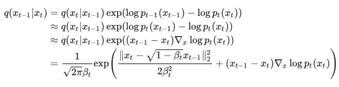
Regarding why the diffusion kernel is a Gaussian transformation, the explanation for the reverse process of the diffusion process also being a Gaussian transformation was intuitively provided in a Zhihu answer by a Tsinghua expert [4]. The second line approximates and . The third line uses a first-order Taylor expansion to eliminate . The fourth line directly substitutes the expression for . Thus, we obtain a Gaussian distribution expression.
▲ The reverse process of diffusion is also a Gaussian distribution
In equations 94 and 125, we modeled the mean of the true Gaussian distribution q as being consistent with our derived expression, and set the variance to be consistent with that of q.
Intuitively, this modeling has many benefits. On one hand, according to the analytical form of KL divergence for two Gaussian distributions, we can eliminate and cancel out most terms, simplifying the modeling. On the other hand, both the true distribution and the approximate distribution depend on . During training, our input is xt, and adopting the same form as the true distribution does not leak any information. Moreover, DDPM has verified that this simplification is indeed feasible in practice.However, the reason this can be done is based on a series of complex mathematical proofs found in papers since 2021. Similarly, quoting the Tsinghua expert’s [4] answer:

▲ The simplification of the Gaussian distribution for denoising in DDPM actually contains profound reasoning
In DDPM, the final optimization objective is rather than . The question remains whether the predicted error is the initial error or the initial error at a certain time step. Who is right or wrong? In fact, this misunderstanding originates from our misunderstanding of the expression regarding .
From equation 63 onwards, several consecutive derivations applied a Gaussian property, namely that the mean and variance of the sum of two independent Gaussian distributions equal the mean and variance of the original distribution. In essence, in the process of applying the reparameterization trick to solve for , we recursively introduced new terms to replace the terms in the recursion. Ultimately, what we obtain is simply a collection of all the noise during the diffusion process. This noise can be referred to as t, or even more accurately, it should not equal any specific time step, but simply be referred to as noise!

▲ The optimization objective of DDPM
Regarding different simplifications of the evidence lower bound, we mentioned that the second method for approximating noise is the modeling approach adopted in DDPM. However, the approximation of the initial input has also been employed by some papers. This is the form utilized in the paper applying diffusion models to controllable text generation mentioned earlier [3]. This paper directly predicts the initial Word-embedding in each round. The third perspective on score-matching can refer to Dr. Song Yang’s series of papers [5]. The optimization function’s form used there is the third one.
This note focuses on the derivation of the variational lower bound formula for diffusion models. It does not cover the relationships between diffusion models and energy models, Langevin dynamics, stochastic differential equations, and other related terms. I plan to organize related understandings in another note.
References
[1] Improving Variational Inference with Inverse Autoregressive Flow https://arxiv.org/abs/1606.04934
[2] Deep Unsupervised Learning using Nonequilibrium Thermodynamics https://arxiv.org/abs/1503.03585
[3] abDiffusion-LM Improves Controllable Text Generation https://arxiv.org/abs/2205.14217
[4] abdiffusion model最近在图像生成领域大红大紫,如何看待它的风头开始超过GAN?- 我想唱high C的回答 – 知乎 https://www.zhihu.com/question/536012286/answer/2533146567
[5] SCORE-BASED GENERATIVE MODELING THROUGH STOCHASTIC DIFFERENTIAL EQUATIONS https://arxiv.org/abs/2011.13456
Editor: Yu Tengkai
Proofreader: Yang Xuejun