A beginner in CV, I write this article to help other novices like me understand how to easily learn and allow experts to reinforce their basics (manual dog head), feel free to leave any questions in the comment section for discussion~
1. Overview
Paper: Densely Connected Convolutional Networks
Paper link: https://arxiv.org/pdf/1608.06993.pdf
As the Best Paper at CVPR 2017, DenseNet breaks away from the conventional thinking of increasing network depth (ResNet) and width (Inception) to improve network performance. From the perspective of features, it significantly reduces the number of parameters through feature reuse and bypass settings, while alleviating the gradient vanishing problem to some extent. With the combination of information flow and feature reuse assumptions, DenseNet rightfully became the Best Paper of the year at the top conference in computer vision in 2017.
Convolutional Neural Networks have become one of the main network structures in deep learning after nearly 20 years of dormancy. From the initial five-layer structure of LeNet, to the later 19-layer structure of VGG, and then to the first networks crossing 100 layers with Highway Networks and ResNet, the deepening of network layers has become one of the main directions of CNN development.
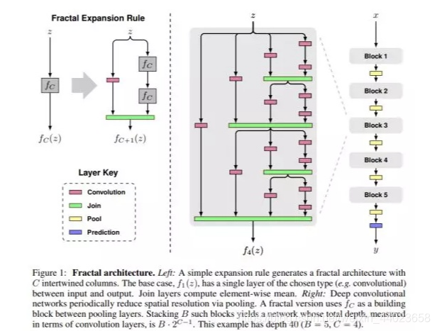
As the number of layers in CNN continues to increase, the gradient vanishing and model degradation problems have emerged. The widespread use of Batch Normalization has alleviated the gradient vanishing problem to some extent, while ResNet and Highway Networks further reduce the occurrence of gradient vanishing and model degradation by constructing identity mappings for bypasses. Fractal Nets parallelize networks of different depths to ensure gradient propagation while gaining depth, and Stochastic Depth demonstrates the redundancy of ResNet’s depth while alleviating the aforementioned problems by randomly deactivating some layers in the network. Although these different network frameworks deepen the network layers through different implementations, they all share the same core idea: connecting feature maps across network layers.
 DenseNet, as another convolutional neural network with a deeper layer count, has the following advantages:
-
(1) Fewer parameters compared to ResNet. -
(2) Bypass enhances feature reuse. -
(3) The network is easier to train and has a certain regularization effect. -
(4) Alleviates the gradient vanishing and model degradation problems.
Mr. Kaiming He made the following assumption when proposing ResNet: If a deeper network has several layers capable of learning identity mappings compared to a shallower network, then the performance of the model trained from this deeper network will not be worse than that of the shallower network.
In simple terms, if we add some layers capable of learning identity mappings to a network, the worst outcome is that these layers in the new network become identity mappings after training, which does not affect the performance of the original network. Similarly, when DenseNet was proposed, it also made an assumption: rather than repeatedly learning redundant features, feature reuse is a better way to extract features.
2. DenseNet
In deep learning networks, as the depth increases, the gradient vanishing problem becomes more pronounced. Many papers have proposed solutions to this problem, such as ResNet, Highway Networks, Stochastic Depth, FractalNets, etc. Despite the structural differences in these algorithms, the core idea is: create short paths from early layers to later layers. So how does the author achieve this? Continuing this idea, all layers are directly connected while ensuring maximum information transfer between layers!
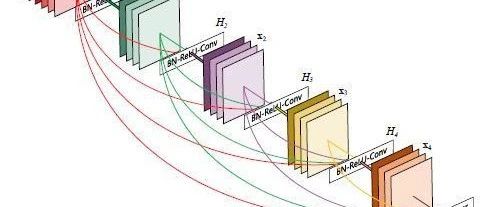
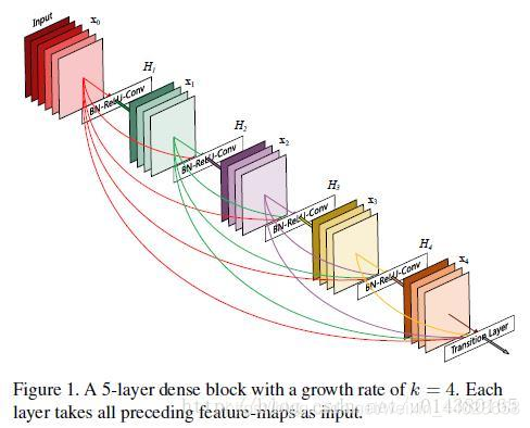
Here is a structure diagram of a dense block. In traditional convolutional neural networks, if you have L layers, there will be L connections, but in DenseNet, there will be L(L+1)/2 connections. In simple terms, each layer’s input comes from the outputs of all previous layers. As shown in the figure: x0 is the input, the input to H1 is x0 (input), the input to H2 is x0 and x1 (where x1 is the output of H1), and so on.
 One advantage of DenseNet is that the network is narrower and has fewer parameters, largely due to this dense block design. It is mentioned later that the number of output feature maps for each convolutional layer in the dense block is small (less than 100), rather than the hundreds or thousands of widths seen in other networks. This connection method also makes feature and gradient transmission more effective, making the network easier to train.
A sentence from the original text that I particularly like: Each layer has direct access to the gradients from the loss function and the original input signal, leading to implicit deep supervision. This directly explains why this network performs so well. As mentioned earlier, the gradient vanishing problem becomes more likely to occur as the network depth increases, due to the transmission of input information and gradient information across many layers. Now, with this dense connection, each layer is directly connected to the input and loss, which can alleviate the gradient vanishing phenomenon, making deeper networks not a problem.
Additionally, the author observed that this dense connection has a regularization effect, thus suppressing overfitting to a certain extent. I believe this is because the parameters are reduced (later I will explain why the parameters are reduced), which lessens the overfitting phenomenon.
This article has the advantage of having almost no formulas, unlike some articles that bombard the reader with complex equations. There are only two formulas in the article, used to illustrate the relationship between DenseNet and ResNet, which are crucial for understanding the principles of these two networks.
-
The first formula is for ResNet. Here, l denotes the layer, xl denotes the output of layer l, and Hl denotes a nonlinear transformation. For ResNet, the output of layer l is the output of layer l-1 plus the nonlinear transformation of the output of layer l-1. -
The second formula is for DenseNet. [x0,x1,…,xl-1] represents the concatenation of the output feature maps from layers 0 to l-1. Concatenation merges the channels, similar to Inception. In contrast, ResNet performs addition, keeping the number of channels unchanged. Hl includes BN, ReLU, and a 3*3 convolution. Thus, from these two formulas, we can see the essential difference between DenseNet and ResNet, which is very insightful.
Next, let’s discuss the Identity function mentioned throughout the paper: it simply means the output equals the input.
The traditional feedforward network structure can be seen as an algorithm for processing network states (feature maps?), where states are transmitted between layers. Each layer reads the state from the previous layer and writes it to the next layer, potentially altering the state or maintaining the transmitted information unchanged. ResNet explicitly uses Identity transformations to convey this invariant information.
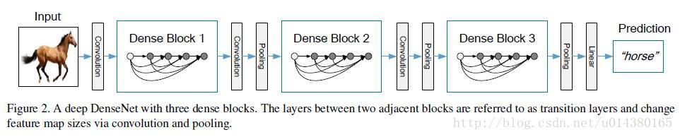
Looking below, Figure 1 represents the dense block, while Figure 2 shows a DenseNet structure diagram, which contains three dense blocks. The author divides DenseNet into multiple dense blocks to ensure that the feature map size within each dense block is uniform, thereby avoiding size issues during concatenation.
 This Table 1 (below) is the overall network structure diagram.
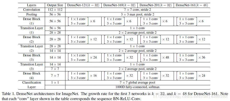
In this table, k=32 and k=48, where k is the growth rate, indicating the number of output feature maps per layer in each dense block. To avoid making the network excessively wide, the author uses a smaller k, such as 32.
The author’s experiments also show that a smaller k can yield better results. According to the design of the dense block, the later layers can obtain the inputs from all previous layers, so the concatenated input channels remain relatively large. Additionally, each dense block’s 3×3 convolution is preceded by a 1×1 convolution operation, which is known as a bottleneck layer. This aims to reduce the number of input feature maps, thereby reducing dimensionality and computation while merging features across channels, which is beneficial.
Furthermore, to further compress parameters, the author adds a 1×1 convolution operation between every two dense blocks. Thus, in the subsequent experimental comparisons, if you see the DenseNet-C network, it indicates that this Translation layer has been added, and the output channel of the 1×1 convolution is set to half of the input channel by default. If you see the DenseNet-BC network, it indicates that it includes both the bottleneck layer and the Translation layer.
Let’s elaborate on the bottleneck and transition layer operations.
Each Dense Block consists of many substructures. Taking the Dense Block (3) of DenseNet-169 as an example, it contains 32 1×1 and 3×3 convolution operations, meaning the input to the 32nd substructure is the output from the previous 31 layers, with the output channel for each layer being 32 (growth rate). If no bottleneck operation is performed, the input to the 32nd layer’s 3×3 convolution would be approximately 1000 due to the concatenation of outputs from the previous Dense Block. However, by adding the 1×1 convolution, the channel in the code is set to the growth rate of 4, which is 128, thus significantly reducing the computational load. This is the bottleneck.
As for the transition layer, it is placed between two Dense Blocks because the output channel count after each Dense Block is quite high. A 1×1 convolution kernel is used to reduce dimensionality. Again, taking the Dense Block (3) of DenseNet-169 as an example, although the output channel of the 32nd layer’s 3×3 convolution is only 32 (growth rate), it will still undergo a channel concatenation operation like previous layers, meaning the input to the 32nd layer is about 1000 channels. Thus, this transition layer has a parameter reduction (ranging from 0 to 1), indicating how much to reduce these outputs. By default, it is set to 0.5, thereby halving the channel count sent to the next Dense Block. The article also uses dropout operations to randomly reduce branches to avoid overfitting, as the connections in this article are indeed numerous.
Experimental Results:
The DenseNet network used by the author varies slightly across different datasets. For example, on the Imagenet dataset, DenseNet-BC has 4 dense blocks, while only 3 dense blocks are used on other datasets. More details can be found in section 3 of the paper, Implementation Details. Training details and hyperparameter settings can be found in section 4.2 of the paper, where a 224*224 center crop is performed during testing on the ImageNet dataset.
Table 2 shows the comparison results of three datasets (C10, C100, SVHN) against other algorithms. ResNet[11] refers to Kaiming He’s paper, and the comparison results are clear at a glance. The network parameters of DenseNet-BC are indeed significantly reduced compared to DenseNet of the same depth! The reduction in parameters not only saves memory but also reduces overfitting. For the SVHN dataset, the results of DenseNet-BC did not perform as well as those of DenseNet (k=24). The author believes this is mainly because the SVHN dataset is relatively simple, and deeper models are prone to overfitting. In the second-to-last area of the table, a comparison of DenseNet with different depths L and k shows that as L and k increase, the model’s performance improves.
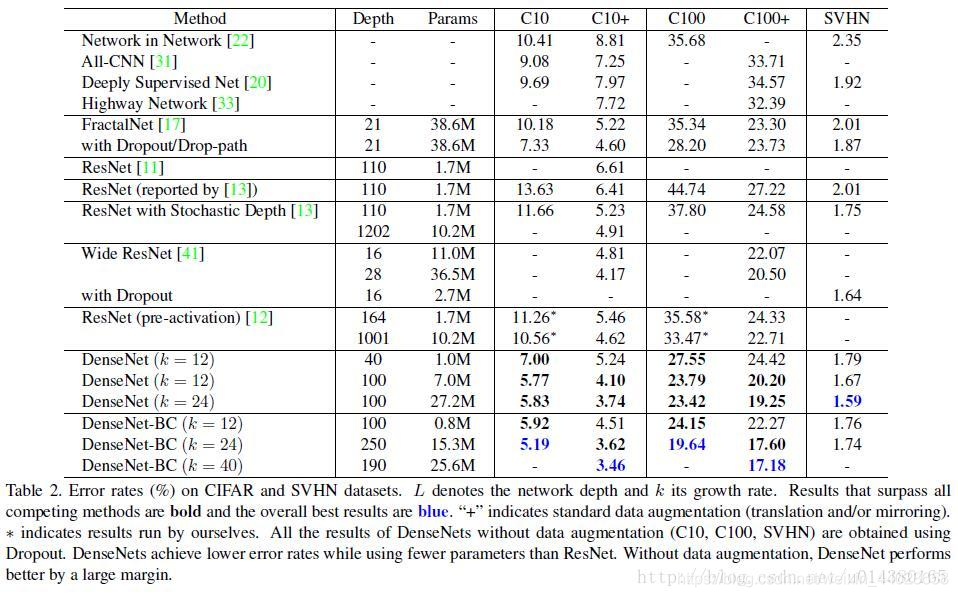 Figure 3 compares DenseNet-BC and ResNet on the Imagenet dataset. The left graph shows the comparison of parameter complexity and error rate. You can observe parameter complexity under the same error rate or error rate under the same parameter complexity, which is significantly improved! The right graph compares flops (which can be understood as computational complexity) and error rate, showing the same effect.
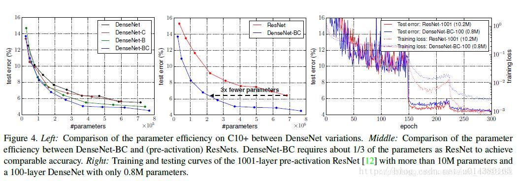
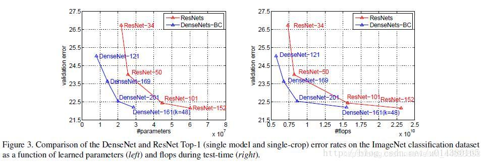 Figure 4 is also important. The left graph illustrates the parameter and error comparison of different types of DenseNet. The middle graph compares DenseNet-BC and ResNet in terms of parameters and error. Under the same error, DenseNet-BC’s parameter complexity is significantly lower. The right graph also shows that DenseNet-BC-100 achieves the same results as ResNet-1001 with very few parameters.
 Initially designed, DenseNet allows each network layer to use all previous layers’ feature maps. To explore the feature reuse situation, the author conducted relevant experiments. The author trained a DenseNet with L=40, K=12, calculating the average absolute value of the weights of the feature maps from a previous layer in the corresponding layer. This average indicates the utilization of a certain layer for the features from a previous layer. The following heatmap is drawn from this average:
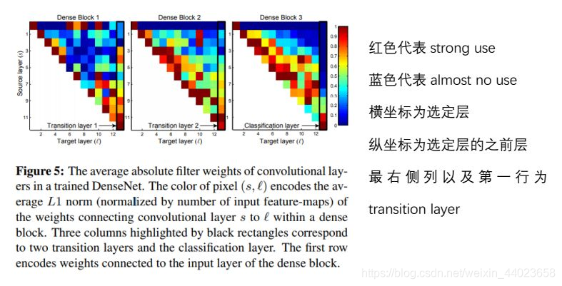 From the figure, we can draw the following conclusions:
-
a Some features extracted from earlier layers may still be directly used by deeper layers. -
b Even Transition layers will utilize features from all layers in the previous Dense block. -
c Layers in the 2nd and 3rd Dense blocks have low utilization of features from previous Transition layers, indicating that the transition layer outputs a large number of redundant features. This also supports the necessity of compression in DenseNet-BC. -
d Although the final classification layer uses information from multiple layers in the previous Dense block, it tends to rely more on features from the last few feature maps, indicating that some high-level features may be generated in the last few layers of the network.
Additionally, it is worth mentioning the relationship between DenseNet and stochastic depth. In stochastic depth, layers in the residual are randomly dropped during training, which essentially creates direct connections between adjacent layers, quite similar to DenseNet.
Conclusion:
The core idea of DenseNet proposed in this article is to establish connections between different layers, fully utilize features, further alleviate the gradient vanishing problem, and make deep networks feasible with excellent training results. Additionally, the use of bottleneck layers, translation layers, and smaller growth rates makes the network narrower, reduces parameters, effectively suppresses overfitting, and decreases computational load. DenseNet has many advantages, and its superiority is very evident in comparison with ResNet.
PyTorch Implementation (Reference from Official DenseNet121)
model.py
The overall structure is as follows:
1. Input: image<br/>2. Pass through feature block (the first convolution layer in the figure, a pooling layer can be added afterward, which is not shown here)<br/>3. Pass through the first dense block, this block contains n dense layers, the gray circles indicate that each dense layer is a dense connection, meaning the input of each layer is the concatenation of outputs from all previous layers.<br/>4. Pass through the first transition block, consisting of convolution and pooling.<br/>5. Pass through the second dense block.<br/>6. Pass through the second transition block.<br/>7. Pass through the third dense block.<br/>8. Pass through the classification block, consisting of pooling and linear layers, outputting softmax scores.<br/>9. Pass through the prediction layer, softmax classification.<br/>10. Output: classification probability.Dense Layer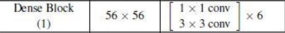 The initial output is (56 * 56 * 64) or the output from the previous dense layer.
1. Batch Normalization, output (56 * 56 * 64)
2. ReLU, output (56 * 56 * 64)
3.
– 1×1 Convolution, kernel_size=1, channel = bn_size * growth_rate, so the output is (56 * 56 * 128)
– Batch Normalization (56 * 56 * 128)
– ReLU (56 * 56 * 128)
4. Convolution, kernel_size=3, channel = growth_rate (56 * 56 * 32)
5. Dropout, optional, used to prevent overfitting (56 * 56 * 32)
class _DenseLayer(nn.Sequential):<br/> def __init__(self, num_input_features, growth_rate, bn_size, drop_rate, memory_efficient=False):#num_input_features feature layer count<br/> super(_DenseLayer, self).__init__()#growth_rate=32 growth rate bn_size=4<br/> # (56 * 56 * 64)<br/> self.add_module('norm1', nn.BatchNorm2d(num_input_features)),<br/> self.add_module('relu1', nn.ReLU(inplace=True)),<br/> self.add_module('conv1', nn.Conv2d(num_input_features, bn_size * growth_rate, kernel_size=1, stride=1, bias=False)),<br/> self.add_module('norm2', nn.BatchNorm2d(bn_size * growth_rate)),<br/> self.add_module('relu2', nn.ReLU(inplace=True)),<br/> self.add_module('conv2', nn.Conv2d(bn_size * growth_rate, growth_rate, kernel_size=3, stride=1, padding=1, bias=False)),<br/> # (56 * 56 * 32)<br/> self.drop_rate = drop_rate<br/> self.memory_efficient = memory_efficient<br/><br/> def forward(self, *prev_features):<br/> bn_function = _bn_function_factory(self.norm1, self.relu1, self.conv1)# (56 * 56 * 64*3)<br/> if self.memory_efficient and any(prev_feature.requires_grad for prev_feature in prev_features):<br/> bottleneck_output = cp.checkpoint(bn_function, *prev_features)<br/> else:<br/> bottleneck_output = bn_function(*prev_features)<br/> # bn1 + relu1 + conv1<br/> new_features = self.conv2(self.relu2(self.norm2(bottleneck_output)))<br/> if self.drop_rate > 0:<br/> new_features = F.dropout(new_features, p=self.drop_rate, training=self.training)<br/> return new_features<br/><br/>def _bn_function_factory(norm, relu, conv):<br/> def bn_function(*inputs):<br/> # type(List[Tensor]) -> Tensor<br/> concated_features = torch.cat(inputs, 1)# merge by channel<br/> # bn1 + relu1 + conv1<br/> bottleneck_output = conv(relu(norm(concated_features)))<br/> return bottleneck_output<br/><br/> return bn_functionDense Block
Dense Block consists of L dense layers.<br/>layer 0: input (56 * 56 * 64) -> output (56 * 56 * 32)<br/>layer 1: input (56 * 56 (32 * 1)) -> output (56 * 56 * 32)<br/>layer 2: input (56 * 56 (32 * 2)) -> output (56 * 56 * 32)<br/>…<br/>layer L: input (56 * 56 * (32 * L)) -> output (56 * 56 * 32)<br/><br/>Note that the output of each L dense layer remains unchanged, while the input channel count increases, as mentioned, each layer's input is the concatenation of all previous layers' outputs.class _DenseBlock(nn.Module):<br/> def __init__(self, num_layers, num_input_features, bn_size, growth_rate, drop_rate, memory_efficient=False):<br/> super(_DenseBlock, self).__init__()# num_layers repetition count<br/> for i in range(num_layers):<br/> layer = _DenseLayer(<br/> num_input_features + i * growth_rate, # increases by 32 for each layer<br/> growth_rate=growth_rate,<br/> bn_size=bn_size,<br/> drop_rate=drop_rate,<br/> memory_efficient=memory_efficient,<br/> )<br/> self.add_module('denselayer%d' % (i + 1), layer) # add denselayer to dictionary<br/><br/> def forward(self, init_features):<br/> features = [init_features] # original feature, 64<br/> for name, layer in self.named_children(): # iteratively traverse the 6 added layers<br/> new_features = layer(*features) # calculate features<br/> features.append(new_features) # append features<br/> return torch.cat(features, 1) # concatenate features by channel 64 + 6*32=256class _Transition(nn.Sequential):<br/> def __init__(self, num_input_features, num_output_features):<br/> super(_Transition, self).__init__()<br/> self.add_module('norm', nn.BatchNorm2d(num_input_features))<br/> self.add_module('relu', nn.ReLU(inplace=True))<br/> self.add_module('conv', nn.Conv2d(num_input_features, num_output_features, kernel_size=1, stride=1, bias=False))<br/> self.add_module('pool', nn.AvgPool2d(kernel_size=2, stride=2))class DenseNet(nn.Module):
r”””Densenet-BC model class, based on
‘”Densely Connected Convolutional Networks” <https://arxiv.org/pdf/1608.06993.pdf>”””
Args:
growth_rate (int) – how many filters to add each layer (`k` in paper)
block_config (list of 4 ints) – how many layers in each pooling block
num_init_features (int) – the number of filters to learn in the first convolution layer
bn_size (int) – multiplicative factor for number of bottle neck layers
(i.e. bn_size * k features in the bottleneck layer)
drop_rate (float) – dropout rate after each dense layer
num_classes (int) – number of classification classes
memory_efficient (bool) – If True, uses checkpointing. Much more memory efficient,
but slower. Default: *False*. See ‘”paper” <https://arxiv.org/pdf/1707.06990.pdf>”””
def __init__(self, growth_rate=32, block_config=(6, 12, 24, 16),
num_init_features=64, bn_size=4, drop_rate=0, num_classes=1000, memory_efficient=False):
super(DenseNet, self).__init__()
# First convolution
self.features = nn.Sequential(OrderedDict([
(‘conv0’, nn.Conv2d(3, num_init_features, kernel_size=7, stride=2,
padding=3, bias=False)),
(‘norm0’, nn.BatchNorm2d(num_init_features)),
(‘relu0’, nn.ReLU(inplace=True)),
(‘pool0’, nn.MaxPool2d(kernel_size=3, stride=2, padding=1)),
]))
# Each denseblock
num_features = num_init_features
for i, num_layers in enumerate(block_config):
block = _DenseBlock(
num_layers=num_layers, # repetition count of layers
num_input_features=num_features, # feature layer count 64
bn_size=bn_size,
growth_rate=growth_rate,
drop_rate=drop_rate, # dropout value 0
memory_efficient=memory_efficient
)
self.features.add_module(‘denseblock%d’ % (i + 1), block) # add denseblock
num_features = num_features + num_layers * growth_rate # update num_features=64+6*32 = 256
if i != len(block_config) – 1:# add a transition layer between every two dense blocks, i != (4-1), i != 3 not the last denseblock, followed by _Transition layer
trans = _Transition(num_input_features=num_features,
num_output_features=num_features // 2) # output channel count halved
self.features.add_module(‘transition%d’ % (i + 1), trans)
num_features = num_features // 2 # update num_features= num_features//2 integer part
# Final batch norm
self.features.add_module(‘norm5’, nn.BatchNorm2d(num_features))
# Linear layer
self.classifier = nn.Linear(num_features, num_classes)
# Official init from torch repo.
for m in self.modules():
if isinstance(m, nn.Conv2d):
nn.init.kaiming_normal_(m.weight)
elif isinstance(m, nn.BatchNorm2d):
nn.init.constant_(m.weight, 1)
nn.init.constant_(m.bias, 0)
elif isinstance(m, nn.Linear):
nn.init.constant_(m.bias, 0)
def forward(self, x):
features = self.features(x) # feature extraction layer
out = F.relu(features, inplace=True)
out = F.adaptive_avg_pool2d(out, (1, 1)) # adaptive average pooling, output size (1, 1)
out = torch.flatten(out, 1)
out = self.classifier(out) # classifier
return out
# def _load_state_dict(model, model_url, progress):
# # ‘.’s are no longer allowed in module names, but previous _DenseLayer
# # has keys ‘norm.1’, ‘relu.1’, ‘conv.1’, ‘norm.2’, ‘relu.2’, ‘conv.2’.
# # They are also in the checkpoints in model_urls. This pattern is used
# # to find such keys.
# pattern = re.compile(
# r’^(.*denselayer\d+\.(?:norm|relu|conv))\.((?:[12])\.(?:weight|bias|running_mean|running_var))$’)
#
# state_dict = load_state_dict_from_url(model_url, progress=progress)
# for key in list(state_dict.keys()):
# res = pattern.match(key)
# if res:
# new_key = res.group(1) + res.group(2)
# state_dict[new_key] = state_dict[key]
# del state_dict[key]
# model.load_state_dict(state_dict)
def _densenet(arch, growth_rate, block_config, num_init_features, pretrained, progress,
**kwargs):
model = DenseNet(growth_rate, block_config, num_init_features, **kwargs)
if pretrained:
_load_state_dict(model, model_urls[arch], progress)
return model
def densenet121(pretrained=False, progress=True, **kwargs):
r”””Densenet-121 model from
‘”Densely Connected Convolutional Networks” <https://arxiv.org/pdf/1608.06993.pdf>”””
Args:
pretrained (bool): If True, returns a model pre-trained on ImageNet
progress (bool): If True, displays a progress bar of the download to stderr
memory_efficient (bool) – If True, uses checkpointing. Much more memory efficient,
but slower. Default: *False*. See ‘”paper” <https://arxiv.org/pdf/1707.06990.pdf>”””
return _densenet(‘densenet121’, 32, (6, 12, 24, 16), 64, pretrained, progress,
**kwargs)
This integrates the entire process.
#model.py<br/><br/>import torch<br/>import torch.nn as nn<br/>import torch.nn.functional as F<br/>import torch.utils.checkpoint as cp<br/>from collections import OrderedDict<br/># from .utils import load_state_dict_from_url<br/><br/>__all__ = ['DenseNet', 'densenet121', 'densenet169', 'densenet201', 'densenet161']<br/><br/><br/>class _DenseLayer(nn.Sequential):<br/> def __init__(self, num_input_features, growth_rate, bn_size, drop_rate, memory_efficient=False):#num_input_features feature layer count<br/> super(_DenseLayer, self).__init__()#growth_rate=32 growth rate bn_size=4<br/> # (56 * 56 * 64)<br/> self.add_module('norm1', nn.BatchNorm2d(num_input_features)),<br/> self.add_module('relu1', nn.ReLU(inplace=True)),<br/> self.add_module('conv1', nn.Conv2d(num_input_features, bn_size * growth_rate, kernel_size=1, stride=1, bias=False)),<br/> self.add_module('norm2', nn.BatchNorm2d(bn_size * growth_rate)),<br/> self.add_module('relu2', nn.ReLU(inplace=True)),<br/> self.add_module('conv2', nn.Conv2d(bn_size * growth_rate, growth_rate, kernel_size=3, stride=1, padding=1, bias=False)),<br/> # (56 * 56 * 32)<br/> self.drop_rate = drop_rate<br/> self.memory_efficient = memory_efficient<br/><br/> def forward(self, *prev_features):<br/> bn_function = _bn_function_factory(self.norm1, self.relu1, self.conv1)# (56 * 56 * 64*3)<br/> if self.memory_efficient and any(prev_feature.requires_grad for prev_feature in prev_features):<br/> bottleneck_output = cp.checkpoint(bn_function, *prev_features)<br/> else:<br/> bottleneck_output = bn_function(*prev_features)<br/> # bn1 + relu1 + conv1<br/> new_features = self.conv2(self.relu2(self.norm2(bottleneck_output)))<br/> if self.drop_rate > 0:<br/> new_features = F.dropout(new_features, p=self.drop_rate, training=self.training)<br/> return new_features<br/><br/>def _bn_function_factory(norm, relu, conv):<br/> def bn_function(*inputs):<br/> # type(List[Tensor]) -> Tensor<br/> concated_features = torch.cat(inputs, 1)# merge by channel<br/> # bn1 + relu1 + conv1<br/> bottleneck_output = conv(relu(norm(concated_features)))<br/> return bottleneck_output<br/><br/> return bn_function<br/><br/>class _DenseBlock(nn.Module):<br/> def __init__(self, num_layers, num_input_features, bn_size, growth_rate, drop_rate, memory_efficient=False):<br/> super(_DenseBlock, self).__init__()# num_layers repetition count<br/> for i in range(num_layers):<br/> layer = _DenseLayer(<br/> num_input_features + i * growth_rate, # increases by 32 for each layer<br/> growth_rate=growth_rate,<br/> bn_size=bn_size,<br/> drop_rate=drop_rate,<br/> memory_efficient=memory_efficient,<br/> )<br/> self.add_module('denselayer%d' % (i + 1), layer) # add denselayer to dictionary<br/><br/> def forward(self, init_features):<br/> features = [init_features] # original feature, 64<br/> for name, layer in self.named_children(): # iteratively traverse the 6 added layers<br/> new_features = layer(*features) # calculate features<br/> features.append(new_features) # append features<br/> return torch.cat(features, 1) # concatenate features by channel 64 + 6*32=256<br/><br/>class _Transition(nn.Sequential):<br/> def __init__(self, num_input_features, num_output_features):<br/> super(_Transition, self).__init__()<br/> self.add_module('norm', nn.BatchNorm2d(num_input_features))<br/> self.add_module('relu', nn.ReLU(inplace=True))<br/> self.add_module('conv', nn.Conv2d(num_input_features, num_output_features, kernel_size=1, stride=1, bias=False))<br/> self.add_module('pool', nn.AvgPool2d(kernel_size=2, stride=2))<br/><br/>class DenseNet(nn.Module):<br/> r"""Densenet-BC model class, based on<br/> '"Densely Connected Convolutional Networks" <https://arxiv.org/pdf/1608.06993.pdf>"""<br/> <br/> Args:<br/> growth_rate (int) - how many filters to add each layer (`k` in paper)<br/> block_config (list of 4 ints) - how many layers in each pooling block<br/> num_init_features (int) - the number of filters to learn in the first convolution layer<br/> bn_size (int) - multiplicative factor for number of bottle neck layers<br/> (i.e. bn_size * k features in the bottleneck layer)<br/> drop_rate (float) - dropout rate after each dense layer<br/> num_classes (int) - number of classification classes<br/> memory_efficient (bool) - If True, uses checkpointing. Much more memory efficient,<br/> but slower. Default: *False*. See '"paper" <https://arxiv.org/pdf/1707.06990.pdf>"""<br/> <br/> def __init__(self, growth_rate=32, block_config=(6, 12, 24, 16),<br/> num_init_features=64, bn_size=4, drop_rate=0, num_classes=1000, memory_efficient=False):<br/> super(DenseNet, self).__init__()<br/> <br/> # First convolution<br/> self.features = nn.Sequential(OrderedDict([<br/> ('conv0', nn.Conv2d(3, num_init_features, kernel_size=7, stride=2,<br/> padding=3, bias=False)),<br/> ('norm0', nn.BatchNorm2d(num_init_features)),<br/> ('relu0', nn.ReLU(inplace=True)),<br/> ('pool0', nn.MaxPool2d(kernel_size=3, stride=2, padding=1)),<br/> ]))<br/> <br/> # Each denseblock<br/> num_features = num_init_features<br/> for i, num_layers in enumerate(block_config):<br/> block = _DenseBlock(<br/> num_layers=num_layers, # repetition count of layers<br/> num_input_features=num_features, # feature layer count 64<br/> bn_size=bn_size,<br/> growth_rate=growth_rate,<br/> drop_rate=drop_rate, # dropout value 0<br/> memory_efficient=memory_efficient<br/> )<br/> self.features.add_module('denseblock%d' % (i + 1), block) # add denseblock<br/> num_features = num_features + num_layers * growth_rate # update num_features=64+6*32 = 256<br/> if i != len(block_config) - 1:# add a transition layer between every two dense blocks, i != (4-1), i != 3 not the last denseblock, followed by _Transition layer<br/> trans = _Transition(num_input_features=num_features,<br/> num_output_features=num_features // 2) # output channel count halved<br/> self.features.add_module('transition%d' % (i + 1), trans)<br/> num_features = num_features // 2 # update num_features= num_features//2 integer part<br/> <br/> # Final batch norm<br/> self.features.add_module('norm5', nn.BatchNorm2d(num_features))<br/> <br/> # Linear layer<br/> self.classifier = nn.Linear(num_features, num_classes)<br/> <br/> # Official init from torch repo.<br/> for m in self.modules():<br/> if isinstance(m, nn.Conv2d):<br/> nn.init.kaiming_normal_(m.weight)<br/> elif isinstance(m, nn.BatchNorm2d):<br/> nn.init.constant_(m.weight, 1)<br/> nn.init.constant_(m.bias, 0)<br/> elif isinstance(m, nn.Linear):<br/> nn.init.constant_(m.bias, 0)<br/> <br/> def forward(self, x):<br/> features = self.features(x) # feature extraction layer<br/> out = F.relu(features, inplace=True)<br/> out = F.adaptive_avg_pool2d(out, (1, 1)) # adaptive average pooling, output size (1, 1)<br/> out = torch.flatten(out, 1)<br/> out = self.classifier(out) # classifier<br/> return out<br/><br/># def _load_state_dict(model, model_url, progress):<br/># # '.'s are no longer allowed in module names, but previous _DenseLayer<br/># # has keys 'norm.1', 'relu.1', 'conv.1', 'norm.2', 'relu.2', 'conv.2'.<br/># # They are also in the checkpoints in model_urls. This pattern is used<br/># # to find such keys.<br/># pattern = re.compile(<br/># r'^(.*denselayer\d+\.(?:norm|relu|conv))\.((?:[12])\.(?:weight|bias|running_mean|running_var))$')<br/># <br/># state_dict = load_state_dict_from_url(model_url, progress=progress)<br/># for key in list(state_dict.keys()):<br/># res = pattern.match(key)<br/># if res:<br/># new_key = res.group(1) + res.group(2)<br/># state_dict[new_key] = state_dict[key]<br/># del state_dict[key]<br/># model.load_state_dict(state_dict)<br/><br/>def _densenet(arch, growth_rate, block_config, num_init_features, pretrained, progress,<br/> **kwargs):<br/> model = DenseNet(growth_rate, block_config, num_init_features, **kwargs)<br/> if pretrained:<br/> _load_state_dict(model, model_urls[arch], progress)<br/> return model<br/><br/>def densenet121(pretrained=False, progress=True, **kwargs):<br/> r"""Densenet-121 model from<br/> '"Densely Connected Convolutional Networks" <https://arxiv.org/pdf/1608.06993.pdf>"""<br/> Args:<br/> pretrained (bool): If True, returns a model pre-trained on ImageNet<br/> progress (bool): If True, displays a progress bar of the download to stderr<br/> memory_efficient (bool) - If True, uses checkpointing. Much more memory efficient,<br/> but slower. Default: *False*. See '"paper" <https://arxiv.org/pdf/1707.06990.pdf>"""<br/> return _densenet('densenet121', 32, (6, 12, 24, 16), 64, pretrained, progress,<br/> **kwargs)<br/>Note: The training set download is explained in detail on the AlexNet blog: https://blog.csdn.net/weixin_44023658/article/details/105798326