1. The Essence of Back Propagation
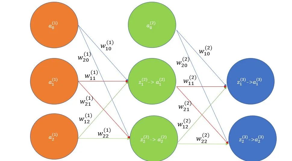
Forward Propagation: Forward propagation is the process by which a neural network transforms input data into prediction results through its hierarchical structure and parameters, achieving complex mappings between input and output.
Forward Propagation
-
Input Layer:
-
The input layer receives sample data from the training set.
-
Each sample contains multiple features, which are passed to the neurons in the input layer.
-
Typically, a bias unit is also added to assist in calculations.
-
Hidden Layer:
-
Each neuron in the hidden layer receives signals from the input layer neurons.
-
These signals are summed after being multiplied by corresponding weights, and a bias is added.
-
Then, the sum is processed by an activation function (such as sigmoid) to produce the hidden layer’s output.
-
Output Layer:
-
The output layer receives signals from the hidden layer and performs similar weighted summation and bias operations.
-
Depending on the problem type, the output layer can directly output these values (for regression problems) or convert them into a probability distribution via an activation function (such as softmax) for classification problems.
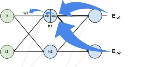
Back Propagation: The backpropagation algorithm uses the chain rule to efficiently compute the error gradients layer by layer from the output layer to the input layer, allowing for the optimization of neural network parameters and minimization of the loss function.
Back Propagation
-
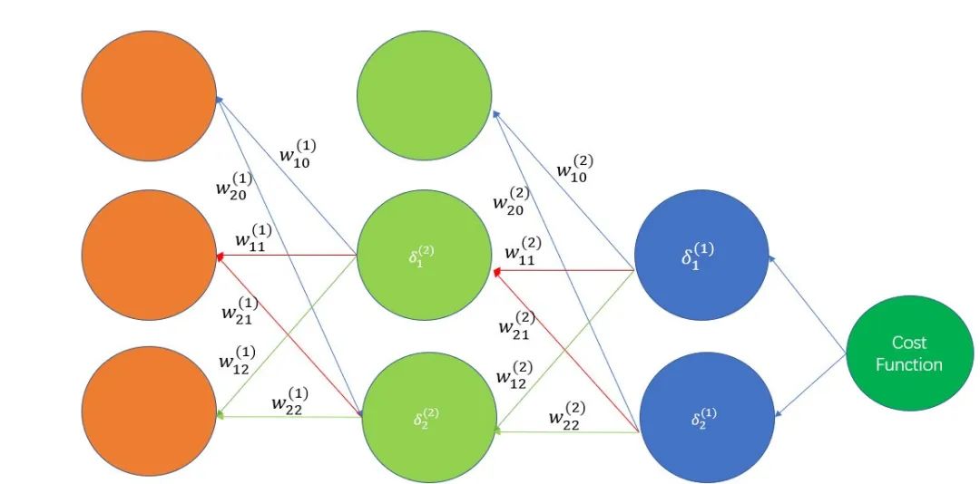
Utilizing the Chain Rule: The backpropagation algorithm is based on the chain rule in calculus, calculating gradients layer by layer to obtain the partial derivatives of parameters in the neural network.
-
Propagation from Output Layer to Input Layer: The algorithm starts from the output layer, calculating the error of the output layer based on the loss function, and then backpropagating the error information to the hidden layer, calculating the error gradients of each neuron layer by layer.
-
Calculating Gradients of Weights and Biases: Using the computed error gradients, the gradients of each weight and bias parameter with respect to the loss function can be further calculated.
-
Parameter Update: Based on the calculated gradient information, gradient descent or other optimization algorithms are used to update the weights and biases in the network to minimize the loss function.
2. The Principles of Back Propagation
Chain Rule: The chain rule is a fundamental theorem in calculus used to compute the derivative of composite functions. If a function is composed of multiple functions, the derivative of that composite function can be calculated by the product of the derivatives of each simple function.
Chain Rule:
-
Simplifying Gradient Calculations: In neural networks, the loss function is typically a composite function formed by the outputs and activation functions of multiple layers. The chain rule allows us to decompose the gradient calculation of this complex composite function into a series of simple local gradient calculations, thereby simplifying the gradient computation process.
-
Efficient Gradient Calculation: By using the chain rule, we can start from the output layer and calculate the gradient of each parameter layer by layer. This layer-by-layer computation avoids redundant calculations and improves the efficiency of gradient computation.
-
Supporting Multi-layer Network Structures: The chain rule applies not only to simple two-layer neural networks but can also be extended to deep neural networks with any number of layers. This enables us to train and optimize more complex models.
Partial Derivatives: Partial derivatives are the result of taking the derivative of a multivariable function with respect to a single variable, and they are used in neural network backpropagation to quantify the sensitivity of the loss function to changes in parameters, guiding parameter optimization.
Definition of Partial Derivatives:
-
Partial derivatives refer to the derivatives taken with respect to one variable in a multivariable function while treating the other variables as constants.
-
In neural networks, partial derivatives quantify the rate of change of the loss function with respect to model parameters (such as weights and biases).
Goal of Back Propagation:
-
The goal of backpropagation is to compute the partial derivatives of the loss function with respect to each parameter so that optimization algorithms (such as gradient descent) can be used to update the parameters.
-
These partial derivatives form the gradient, guiding the direction and magnitude of parameter updates.
Computation Process:
-
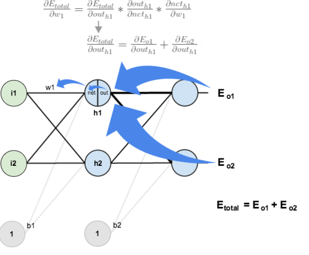
Partial Derivative of Output Layer: First, compute the partial derivative of the loss function with respect to the output of the output layer neurons. This typically depends directly on the chosen loss function.
-
Partial Derivative of Hidden Layer: Using the chain rule, backpropagate the partial derivatives from the output layer to the hidden layer. For each neuron in the hidden layer, calculate its output with respect to the input of the next layer and multiply it by the partial derivative returned from the next layer to accumulate the total partial derivative of that neuron with respect to the loss function.
-
Parameter Partial Derivatives: After calculating the partial derivatives for the output and hidden layers, we further compute the partial derivatives of the loss function with respect to the network parameters, i.e., the weights and biases.
3. Case Study of Back Propagation: Simple Neural Network
1. Network Structure
-
Assuming we have a simple two-layer neural network structured as follows:
-
Input Layer: 2 neurons (input features x1 and x2)
-
Hidden Layer: 2 neurons (with sigmoid activation function)
-
Output Layer: 1 neuron (with sigmoid activation function)
-
The weights and biases of the network are as follows (these values are randomly initialized; in practice, random initialization will be used):
-
Weight matrix W1 from input layer to hidden layer: [[0.5, 0.3], [0.2, 0.4]]
-
Weight vector W2 from hidden layer to output layer: [0.6, 0.7]
-
Bias vector b1 for hidden layer: [0.1, 0.2]
-
Bias b2 for output layer: 0.3
2. Forward Propagation
-
Given input
[0.5, 0.3], perform forward propagation: -
Hidden layer input:
[0.5*0.5 + 0.3*0.2 + 0.1, 0.5*0.3 + 0.3*0.4 + 0.2]=[0.31, 0.29] -
Hidden layer output (after sigmoid activation function):
[sigmoid(0.31), sigmoid(0.29)]≈[0.57, 0.57] -
Output layer input:
0.6*0.57 + 0.7*0.57 + 0.3=0.71 -
Output layer output (prediction value, after sigmoid activation function):
sigmoid(0.71)≈0.67
3. Loss Calculation
-
Assuming the true label is
0.8, calculate the loss using Mean Squared Error (MSE): -
Loss =
(0.8 - 0.67)^2≈0.017
4. Back Propagation: Calculate the partial derivatives of the loss function with respect to the network parameters and backpropagate the error starting from the output layer.
-
Output Layer Partial Derivative:
-
Partial derivative of the loss function with respect to the output layer input (δ2):
2 * (0.67 - 0.8) * sigmoid_derivative(0.71)≈-0.05 -
The derivative of the sigmoid function:
sigmoid(x) * (1 - sigmoid(x)) -
Hidden Layer Partial Derivative:
-
Partial derivatives of the loss function with respect to each neuron output in the hidden layer (δ1):
[δ2 * 0.6 * sigmoid_derivative(0.31), δ2 * 0.7 * sigmoid_derivative(0.29)] -
After calculation, δ1 ≈
[-0.01, -0.01](simplified for clarity; actual values may differ) -
Parameter Partial Derivatives:
-
For weights W2:
[δ2 * hidden_layer_output1, δ2 * hidden_layer_output2]=[-0.03, -0.04] -
For bias b2:
δ2=-0.05 -
For weights W1 and biases b1, more complex calculations are required as they influence the hidden layer output, which in turn affects the input to the output layer and the final loss. These partial derivatives depend on δ1 and the values from the input layer.
5. Parameter Update
-
Use gradient descent to update parameters (learning rate set to 0.1):
-
Update W2:
W2 - learning_rate * parameter_partial_derivative -
Update b2:
b2 - learning_rate * parameter_partial_derivative -
Similarly update W1 and b1
6. Iteration
-
Repeat steps 2-5 until the network converges or a preset number of iterations is reached.