
Source: Machine Learning Algorithms<br/><br/> This article is approximately 6500 words long and is suggested to take 13 minutes to read. This article provides a complete introduction to the necessary knowledge about diffusion models and implements it fully using PyTorch.
The trigger for diffusion models began with the introduction of the Denoising Diffusion Probabilistic Model (DDPM) in 2020. Before diving into the details of how the denoising diffusion probabilistic model (DDPM) works, let’s first look at some developments in existing generative artificial intelligence, which are foundational studies for DDPM:
VAE
VAEs utilize an encoder, a probabilistic latent space, and a decoder. During training, the encoder predicts the mean and variance for each image. Then, samples are drawn from a Gaussian distribution based on these values and passed to the decoder, where the input image is expected to resemble the output image. This process involves using KL Divergence to calculate loss. One significant advantage of VAEs is their ability to generate a wide variety of images. During the sampling phase, simply sampling from the Gaussian distribution, the decoder creates a new image.
GAN
Just a year after the introduction of Variational Autoencoders (VAEs), a groundbreaking generative family model emerged – Generative Adversarial Networks (GANs), marking the beginning of a new class of generative models characterized by the collaboration of two neural networks: a generator and a discriminator, involving an adversarial training process. The generator aims to generate real data, such as images, from random noise, while the discriminator strives to distinguish between real and generated data. Throughout the training phase, the generator and discriminator continuously refine their capabilities through a competitive learning process. The generator generates increasingly convincing data, becoming smarter than the discriminator, while the discriminator improves its ability to distinguish between real and generated samples. This adversarial interaction peaks when the generator produces high-quality, realistic data. In the sampling phase, after GAN training, the generator produces new samples by inputting random noise, converting this noise into data that typically reflects real examples.
Why We Need Diffusion Models: DDPM
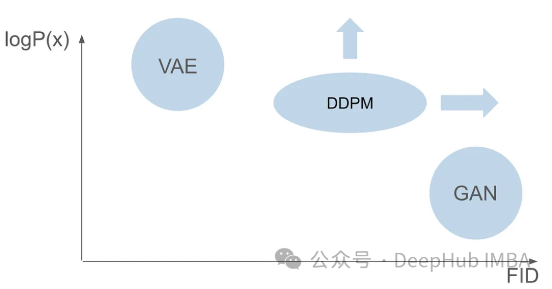
Both models have different issues; while GANs excel at generating realistic images that are very similar to those in the training set, VAEs are adept at creating a wide variety of images, although they tend to produce blurry images. However, existing models have not successfully combined these two functionalities—creating images that are both highly realistic and diverse. This challenge presents a significant barrier for researchers to overcome.
Six years after the first GAN paper was published and seven years after the VAE paper, a groundbreaking model emerged: the Denoising Diffusion Probabilistic Model (DDPM). DDPM combines the advantages of both models and excels at creating diverse and realistic images.
In this article, we will delve into the complexities of DDPM, covering its training process, including forward and reverse processes, and explore how to perform sampling. Throughout this exploration, we will build DDPM from scratch using PyTorch and complete its full training.
It is assumed that you are already familiar with the fundamentals of deep learning and have a solid foundation in deep computer vision. We will not introduce these basic concepts; our goal is to generate images that humans are convinced of their authenticity.
Diffusion Model DDPM
The Denoising Diffusion Probabilistic Model (DDPM) is a cutting-edge method in the field of generative models. Unlike traditional models that rely on explicit likelihood functions, DDPM operates by iteratively denoising through a diffusion process. This involves gradually adding noise to images and attempting to remove that noise. Its fundamental theory is based on the idea that by transforming a simple distribution, such as a Gaussian distribution, through a series of diffusion steps, a complex and expressive image data distribution can be obtained. In other words, by transferring samples from the original image distribution to the Gaussian distribution, we can create a model to reverse this process. This enables us to start from a fully Gaussian distribution and end with an image distribution, effectively generating new images.
The training of DDPM involves two fundamental steps: generating noisy images, which is a fixed and non-learnable forward process, and the subsequent reverse process. The main goal of the reverse process is to denoise the images using a specialized machine learning model.
Forward Diffusion Process
The forward process is a fixed and non-learnable step, but it requires some predefined settings. Before delving into these settings, let’s first understand how it works.
The core concept of this process starts with a clear image. At specific time steps denoted by “T,” a small amount of noise is gradually introduced according to a Gaussian distribution.
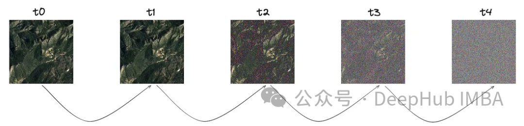
From the image, it can be seen that noise is incrementally added at each step, and we will delve into the mathematical representation of this noise.
The noise is sampled from a Gaussian distribution. To introduce a small amount of noise at each step, we use a Markov chain. To generate the image at the current timestamp, we only need the image from the last timestamp. The concept of the Markov chain is crucial here and is essential for the subsequent mathematical details.
A Markov chain is a stochastic process where the probability of transitioning to any specific state depends only on the current state and the elapsed time, rather than the sequence of events that preceded it. This property simplifies the modeling of the noise addition process, making it easier for mathematical analysis.

The variance parameter denoted by beta is intentionally set to a very small value, aiming to introduce only a minimal amount of noise at each step.
The step parameter “T” determines the number of steps required to generate a fully noisy image. In this article, this parameter is set to 1000, which may seem large. Do we really need to create 1000 noisy images for each original image in the dataset? The aspect of the Markov chain proves to be helpful in addressing this issue. Since we only need the previous image to predict the next one, and the noise added at each step remains unchanged, we can simplify the computation by generating noisy images at specific timestamps. The right reparameterization technique allows us to further simplify the equations.
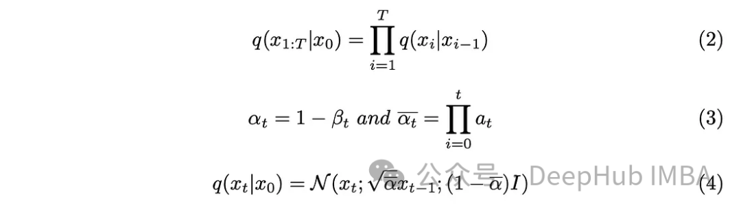
Introducing the new parameters from equation (3) into equation (2) develops equation (2) into the desired result.
Reverse Diffusion Process
Now that we have introduced noise to the images, the next step is to perform the reverse operation. Mathematically, we cannot implement the denoising of the image unless we know the initial conditions, specifically the denoised image at t = 0. Our goal is to sample directly from the noise to create new images, where there is a lack of information about the result. Therefore, I need to design a method to gradually denoise the image without knowing the outcome. This leads to the solution of using deep learning models to approximate this complex mathematical function.
With a bit of mathematical background, the model will approximate equation (5). A noteworthy detail is that we will adhere to the original DDPM paper and keep the variance fixed, even though it is also possible to allow the model to learn it.

The task of the model is to predict the average noise added between the current timestamp and the previous timestamp. Doing so effectively removes the noise, achieving the desired effect. But what if our goal is for the model to predict the noise added from the “original image” to the last timestamp?
Mathematically, executing the reverse process is challenging unless we know the initial image without noise, so let’s start by defining the posterior variance.
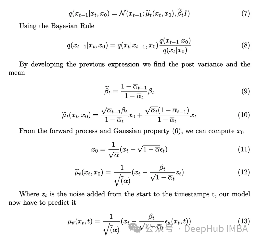
The model’s task is to predict the noise of the image added at timestamp t from the initial image. The forward process allows us to perform this operation, starting from a clear image and progressing to a noisy image at timestamp t.
Training Algorithm
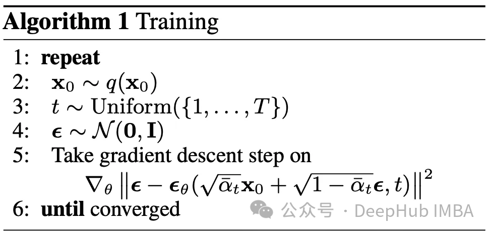
We assume that the model architecture used for predictions will be a U-Net. The objective during the training phase is: for each image in the dataset, randomly select a timestamp in the range [0,T] and compute the forward diffusion process. This generates a clear, slightly noisy image, along with the actual noise used. Then, leveraging our understanding of the reverse process, we use the model to predict the noise added to the image. With both true and predicted noise, we seem to have entered a supervised machine learning problem.
The main question arises: which loss function should we use to train our model? Since we are dealing with a probabilistic latent space, Kullback-Leibler (KL) divergence is a suitable choice.
KL divergence measures the difference between two probability distributions, in our case, the distribution predicted by the model and the expected distribution. Including KL divergence in the loss function not only guides the model to produce accurate predictions but also ensures that the latent space representation conforms to the expected probabilistic structure.
KL divergence can be approximated as an L2 loss function, leading to the following loss function:

Ultimately, we arrive at the training algorithm proposed in the paper.
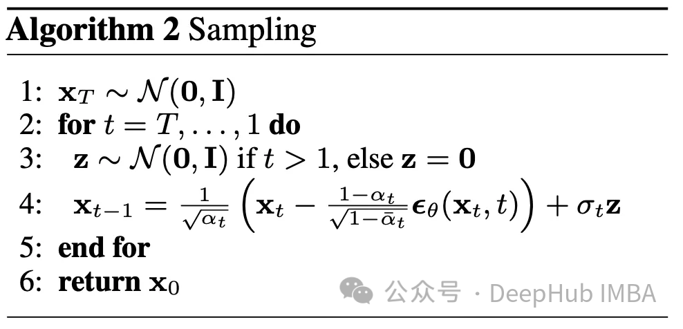
Sampling
The reverse process has been explained; now let’s see how to use it. Starting from a completely random image at time T and using the reverse process T times, we ultimately arrive at time 0. This constitutes the second algorithm outlined in this article.
Parameters
We have many different parameters like beta, beta_tildes, alpha, alpha_hat, etc. Currently, it is unknown how to choose these parameters. However, the only known parameter at this time is T, which is set to 1000.
For all listed parameters, their selection depends on beta. In a sense, beta determines the amount of noise we want to add at each step. Therefore, careful selection of beta is crucial for the success of the algorithm. For the other parameters, due to their abundance, please refer to the paper.
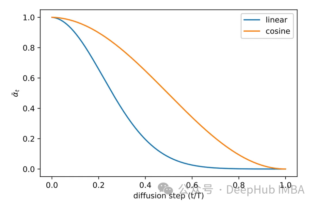
Various sampling methods were explored in the experimental phase of the original paper. The initial linear sampling method resulted in images that either received insufficient noise or became overly noisy. To address this issue, another more commonly used method, cosine sampling, was adopted. Cosine sampling provides smoother and more consistent noise addition.
Implementing the Diffusion Model in PyTorch
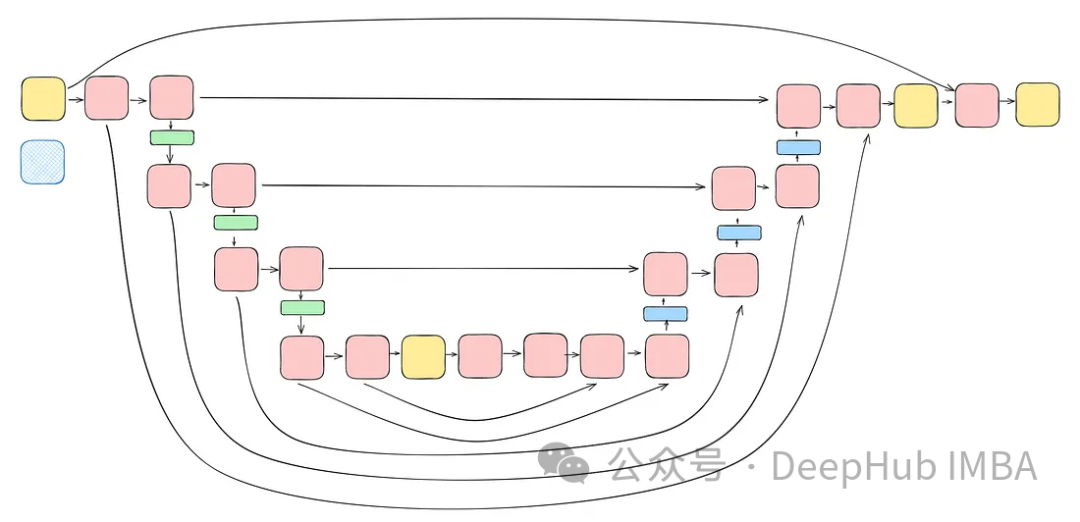
We will utilize the U-Net architecture for noise prediction, as U-Net is an ideal architecture for image processing, capturing spatial and feature maps, and providing output sizes that match the input.
Given the complexity of the task and the requirement to use the same model at each step (where the model needs to denoise completely noisy images and slightly noisy images with the same weights), adjusting the model is essential. This includes merging more complex blocks and introducing sinusoidal embeddings to provide awareness of the timestamps used. The aim of these enhancements is to make the model an expert in denoising tasks. Before continuing to build the complete model, we will introduce each block.
ConvNext Block
To meet the need for increased model complexity, convolutional blocks play a crucial role. We cannot merely rely on the basic blocks from the U-Net paper; we will integrate ConvNext.
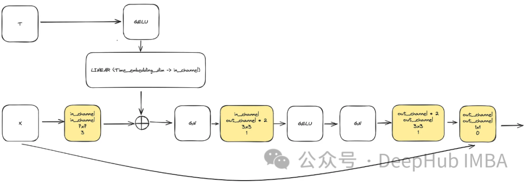
The input consists of “x” representing the image and a timestamp embedding of size “time_embedding_dim” denoted as “t.” Due to the complexity of the blocks and the residual connections with the input and final layer, the blocks play a key role in learning spatial and feature mappings throughout the process.
class ConvNextBlock(nn.Module): def __init__( self, in_channels, out_channels, mult=2, time_embedding_dim=None, norm=True, group=8, ): super().__init__() self.mlp = ( nn.Sequential(nn.GELU(), nn.Linear(time_embedding_dim, in_channels)) if time_embedding_dim else None ) self.in_conv = nn.Conv2d( in_channels, in_channels, 7, padding=3, groups=in_channels ) self.block = nn.Sequential( nn.GroupNorm(1, in_channels) if norm else nn.Identity(), nn.Conv2d(in_channels, out_channels * mult, 3, padding=1), nn.GELU(), nn.GroupNorm(1, out_channels * mult), nn.Conv2d(out_channels * mult, out_channels, 3, padding=1), ) self.residual_conv = ( nn.Conv2d(in_channels, out_channels, 1) if in_channels != out_channels else nn.Identity() ) def forward(self, x, time_embedding=None): h = self.in_conv(x) if self.mlp is not None and time_embedding is not None: assert self.mlp is not None, "MLP is None" h = h + rearrange(self.mlp(time_embedding), "b c -> b c 1 1") h = self.block(h) return h + self.residual_conv(x)Sinusoidal Timestamp Embedding
One of the key blocks in the model is the sinusoidal timestamp embedding block, which allows the encoding of a given timestamp to retain information about the current time required for the model to decode, as this model will be used for all different timestamps.
This is a very classic implementation and applied in various places, so we will directly provide the code.
class SinusoidalPosEmb(nn.Module): def __init__(self, dim, theta=10000): super().__init__() self.dim = dim self.theta = theta def forward(self, x): device = x.device half_dim = self.dim // 2 emb = math.log(self.theta) / (half_dim - 1) emb = torch.exp(torch.arange(half_dim, device=device) * -emb) emb = x[:, None] * emb[None, :] emb = torch.cat((emb.sin(), emb.cos()), dim=-1) return embDownSample & UpSample
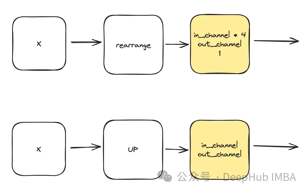
class DownSample(nn.Module): def __init__(self, dim, dim_out=None): super().__init__() self.net = nn.Sequential( Rearrange("b c (h p1) (w p2) -> b (c p1 p2) h w", p1=2, p2=2), nn.Conv2d(dim * 4, default(dim_out, dim), 1), ) def forward(self, x): return self.net(x) class Upsample(nn.Module): def __init__(self, dim, dim_out=None): super().__init__() self.net = nn.Sequential( nn.Upsample(scale_factor=2, mode="nearest"), nn.Conv2d(dim, dim_out or dim, kernel_size=3, padding=1), ) def forward(self, x): return self.net(x)Time Multi-Layer Perceptron
This module utilizes it to create time representations based on the given timestamp t. The output of this multi-layer perceptron (MLP) will also serve as the input “t” for all modified ConvNext blocks.
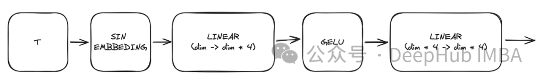
Here, “dim” is a hyperparameter of the model that represents the number of channels required for the first block. It serves as the basis for calculating the number of channels in subsequent blocks.
sinu_pos_emb = SinusoidalPosEmb(dim, theta=10000) time_dim = dim * 4 time_mlp = nn.Sequential( sinu_pos_emb, nn.Linear(dim, time_dim), nn.GELU(), nn.Linear(time_dim, time_dim), )Attention
This is an optional component used in U-Net. Attention helps enhance the role of residual connections in learning. It focuses more on important spatial information obtained from the left side of U-Net through a residual connection and a feature map computed in low latent space. It originates from the ACC-UNet paper.
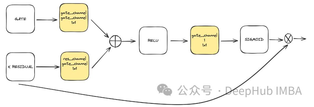
gate represents the upsample output of the lower block, while x residual represents the residual connection at the level where attention is applied.
class BlockAttention(nn.Module): def __init__(self, gate_in_channel, residual_in_channel, scale_factor): super().__init__() self.gate_conv = nn.Conv2d(gate_in_channel, gate_in_channel, kernel_size=1, stride=1) self.residual_conv = nn.Conv2d(residual_in_channel, gate_in_channel, kernel_size=1, stride=1) self.in_conv = nn.Conv2d(gate_in_channel, 1, kernel_size=1, stride=1) self.relu = nn.ReLU() self.sigmoid = nn.Sigmoid() def forward(self, x: torch.Tensor, g: torch.Tensor) -> torch.Tensor: in_attention = self.relu(self.gate_conv(g) + self.residual_conv(x)) in_attention = self.in_conv(in_attention) in_attention = self.sigmoid(in_attention) return in_attention * xFinal Integration
Integrate all the blocks discussed earlier (excluding the attention block) into a U-Net. Each block contains two residual connections instead of one. This modification is intended to address potential overfitting issues.
class TwoResUNet(nn.Module): def __init__( self, dim, init_dim=None, out_dim=None, dim_mults=(1, 2, 4, 8), channels=3, sinusoidal_pos_emb_theta=10000, convnext_block_groups=8, ): super().__init__() self.channels = channels input_channels = channels self.init_dim = default(init_dim, dim) self.init_conv = nn.Conv2d(input_channels, self.init_dim, 7, padding=3) dims = [self.init_dim, *map(lambda m: dim * m, dim_mults)] in_out = list(zip(dims[:-1], dims[1:])) sinu_pos_emb = SinusoidalPosEmb(dim, theta=sinusoidal_pos_emb_theta) time_dim = dim * 4 self.time_mlp = nn.Sequential( sinu_pos_emb, nn.Linear(dim, time_dim), nn.GELU(), nn.Linear(time_dim, time_dim), ) self.downs = nn.ModuleList([]) self.ups = nn.ModuleList([]) num_resolutions = len(in_out) for ind, (dim_in, dim_out) in enumerate(in_out): is_last = ind >= (num_resolutions - 1) self.downs.append( nn.ModuleList( [ ConvNextBlock( in_channels=dim_in, out_channels=dim_in, time_embedding_dim=time_dim, group=convnext_block_groups, ), ConvNextBlock( in_channels=dim_in, out_channels=dim_in, time_embedding_dim=time_dim, group=convnext_block_groups, ), DownSample(dim_in, dim_out) if not is_last else nn.Conv2d(dim_in, dim_out, 3, padding=1), ] ) ) mid_dim = dims[-1] self.mid_block1 = ConvNextBlock(mid_dim, mid_dim, time_embedding_dim=time_dim) self.mid_block2 = ConvNextBlock(mid_dim, mid_dim, time_embedding_dim=time_dim) for ind, (dim_in, dim_out) in enumerate(reversed(in_out)): is_last = ind == (len(in_out) - 1) is_first = ind == 0 self.ups.append( nn.ModuleList( [ ConvNextBlock( in_channels=dim_out + dim_in, out_channels=dim_out, time_embedding_dim=time_dim, group=convnext_block_groups, ), ConvNextBlock( in_channels=dim_out + dim_in, out_channels=dim_out, time_embedding_dim=time_dim, group=convnext_block_groups, ), Upsample(dim_out, dim_in) if not is_last else nn.Conv2d(dim_out, dim_in, 3, padding=1) ] ) ) default_out_dim = channels self.out_dim = default(out_dim, default_out_dim) self.final_res_block = ConvNextBlock(dim * 2, dim, time_embedding_dim=time_dim) self.final_conv = nn.Conv2d(dim, self.out_dim, 1) def forward(self, x, time): b, _, h, w = x.shape x = self.init_conv(x) r = x.clone() t = self.time_mlp(time) unet_stack = [] for down1, down2, downsample in self.downs: x = down1(x, t) unet_stack.append(x) x = down2(x, t) unet_stack.append(x) x = downsample(x) x = self.mid_block1(x, t) x = self.mid_block2(x, t) for up1, up2, upsample in self.ups: x = torch.cat((x, unet_stack.pop()), dim=1) x = up1(x, t) x = torch.cat((x, unet_stack.pop()), dim=1) x = up2(x, t) x = upsample(x) x = torch.cat((x, r), dim=1) x = self.final_res_block(x, t) return self.final_conv(x)Code Implementation of Diffusion
Finally, we will introduce how diffusion is implemented. Since we have already covered all the mathematical theories for the forward, reverse, and sampling processes, we will focus here on the code.
class DiffusionModel(nn.Module): SCHEDULER_MAPPING = { "linear": linear_beta_schedule, "cosine": cosine_beta_schedule, "sigmoid": sigmoid_beta_schedule, } def __init__( self, model: nn.Module, image_size: int, *, beta_scheduler: str = "linear", timesteps: int = 1000, schedule_fn_kwargs: dict | None = None, auto_normalize: bool = True, ) -> None: super().__init__() self.model = model self.channels = self.model.channels self.image_size = image_size self.beta_scheduler_fn = self.SCHEDULER_MAPPING.get(beta_scheduler) if self.beta_scheduler_fn is None: raise ValueError(f"unknown beta schedule {beta_scheduler}") if schedule_fn_kwargs is None: schedule_fn_kwargs = {} betas = self.beta_scheduler_fn(timesteps, **schedule_fn_kwargs) alphas = 1.0 - betas alphas_cumprod = torch.cumprod(alphas, dim=0) alphas_cumprod_prev = F.pad(alphas_cumprod[:-1], (1, 0), value=1.0) posterior_variance = ( betas * (1.0 - alphas_cumprod_prev) / (1.0 - alphas_cumprod) ) register_buffer = lambda name, val: self.register_buffer( name, val.to(torch.float32) ) register_buffer("betas", betas) register_buffer("alphas_cumprod", alphas_cumprod) register_buffer("alphas_cumprod_prev", alphas_cumprod_prev) register_buffer("sqrt_recip_alphas", torch.sqrt(1.0 / alphas)) register_buffer("sqrt_alphas_cumprod", torch.sqrt(alphas_cumprod)) register_buffer( "sqrt_one_minus_alphas_cumprod", torch.sqrt(1.0 - alphas_cumprod) ) register_buffer("posterior_variance", posterior_variance) timesteps, *_ = betas.shape self.num_timesteps = int(timesteps) self.sampling_timesteps = timesteps self.normalize = normalize_to_neg_one_to_one if auto_normalize else identity self.unnormalize = unnormalize_to_zero_to_one if auto_normalize else identity @torch.inference_mode() def p_sample(self, x: torch.Tensor, timestamp: int) -> torch.Tensor: b, *_, device = *x.shape, x.device batched_timestamps = torch.full( (b,), timestamp, device=device, dtype=torch.long ) preds = self.model(x, batched_timestamps) betas_t = extract(self.betas, batched_timestamps, x.shape) sqrt_recip_alphas_t = extract( self.sqrt_recip_alphas, batched_timestamps, x.shape ) sqrt_one_minus_alphas_cumprod_t = extract( self.sqrt_one_minus_alphas_cumprod, batched_timestamps, x.shape ) predicted_mean = sqrt_recip_alphas_t * ( x - betas_t * preds / sqrt_one_minus_alphas_cumprod_t ) if timestamp == 0: return predicted_mean else: posterior_variance = extract( self.posterior_variance, batched_timestamps, x.shape ) noise = torch.randn_like(x) return predicted_mean + torch.sqrt(posterior_variance) * noise @torch.inference_mode() def p_sample_loop( self, shape: tuple, return_all_timesteps: bool = False ) -> torch.Tensor: batch, device = shape[0], "mps" img = torch.randn(shape, device=device) for t in tqdm(reversed(range(0, self.num_timesteps)), total=self.num_timesteps): img = self.p_sample(img, t) ret = img ret = self.unnormalize(ret) return ret def sample( self, batch_size: int = 16, return_all_timesteps: bool = False ) -> torch.Tensor: shape = (batch_size, self.channels, self.image_size, self.image_size) return self.p_sample_loop(shape, return_all_timesteps=return_all_timesteps) def q_sample( self, x_start: torch.Tensor, t: int, noise: torch.Tensor = None ) -> torch.Tensor: if noise is None: noise = torch.randn_like(x_start) sqrt_alphas_cumprod_t = extract(self.sqrt_alphas_cumprod, t, x_start.shape) sqrt_one_minus_alphas_cumprod_t = extract( self.sqrt_one_minus_alphas_cumprod, t, x_start.shape ) return sqrt_alphas_cumprod_t * x_start + sqrt_one_minus_alphas_cumprod_t * noise def p_loss( self, x_start: torch.Tensor, t: int, noise: torch.Tensor = None, loss_type: str = "l2", ) -> torch.Tensor: if noise is None: noise = torch.randn_like(x_start) x_noised = self.q_sample(x_start, t, noise=noise) predicted_noise = self.model(x_noised, t) if loss_type == "l2": loss = F.mse_loss(noise, predicted_noise) elif loss_type == "l1": loss = F.l1_loss(noise, predicted_noise) else: raise ValueError(f"unknown loss type {loss_type}") return loss def forward(self, x: torch.Tensor) -> torch.Tensor: b, c, h, w, device, img_size = *x.shape, x.device, self.image_size assert h == w == img_size, f"image size must be {img_size}" timestamp = torch.randint(0, self.num_timesteps, (1,)).long().to(device) x = self.normalize(x) return self.p_loss(x, timestamp)The diffusion process is the model’s training component. It opens up a sampling interface that allows us to generate samples using the already trained model.
Summary of Training Points
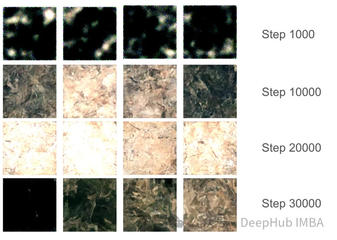
For the training part, we set up 37,000 training steps with a batch size of 16. Due to GPU memory allocation limits, the image size is restricted to 128×128. Using Exponential Moving Average (EMA) model weights, samples are generated every 1000 steps to smooth the sampling and save model versions.
In the initial 1000 training steps, the model began to capture some features but still missed certain areas. Around 10,000 steps, the model started to produce promising results, and progress became more apparent. By the final 30,000 steps, the quality of the results significantly improved, but there were still black images. This was simply because the model did not have enough sample variety; the data distribution of real images did not fully map to the Gaussian distribution.
With the final model weights, we can generate some images. Although the image quality is limited due to the 128×128 size restriction, the model’s performance is still commendable.

Note: The dataset used in this article consists of satellite images of forest terrain; for specific acquisition methods, please refer to the ETL section in the source code.
Conclusion
We have comprehensively introduced the necessary knowledge about diffusion models and fully implemented it using PyTorch.
Editor: Yu Tengkai
Proofreader: Lin Yilin