
Source: DeepHub IMBA


This article is about 2000 words long and is recommended to be read in 5 minutes.
This article will introduce some basic tensor operations in PyTorch.
PyTorch is a scientific computing package based on Python. Its flexibility allows for easy integration of new data types and algorithms, and the framework is also efficient and scalable. Below, we will introduce some basic tensor operations in PyTorch.

Tensors
Tensors are a vector, matrix, or any n-dimensional array. They are the fundamental data structure in deep learning, very similar to arrays and matrices, allowing us to efficiently perform mathematical operations on large datasets. Tensors can be represented as matrices, vectors, scalars, or high-dimensional arrays.
We can think of tensors as simple arrays containing scalars or other arrays. In PyTorch, tensors are a structure very similar to ndarrays, with the difference that they can run on a GPU, greatly accelerating the computation process.
1. tensor()
We generally use the tensor() method to create tensors:
torch.tensor([[3, 6], [2, 4.]]) tensor([[3., 6.], [2., 4.]])Here, it is important to ensure that the dimensions of the Python array passed are the same; for example, the following will raise an error.
torch.tensor([[1, 2], [3, 4, 5]])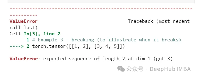
2. randint()
The randint() method returns a tensor filled with random integers uniformly distributed between low (inclusive) and high (exclusive) of the given shape. The shape can be a tuple or a list containing non-negative members. The default value of low is 0. When only one int parameter is passed, low defaults to 0, and high takes the passed value.
torch.randint(2,5, (2,2)) tensor([[2, 4], [2, 4]])3. complex()
The complex() method takes two parameters (real and imaginary) and returns a complex tensor, where the real part is real, and the imaginary part is imaginary, both of which are tensors of the same data type and shape.
 a_real = torch.rand(2, 2) print(a_real) a_imag = torch.rand(2, 2) print(a_imag) a_complex_tensor = torch.complex(a_real, a_imag) print(a_complex_tensor)
tensor([[0.4356, 0.7506],        [0.5335, 0.6262]]) tensor([[0.1342, 0.0804],        [0.2047, 0.0685]]) tensor([[0.4356+0.1342j, 0.7506+0.0804j],        [0.5335+0.2047j, 0.6262+0.0685j]])
If the shapes of the real and imaginary parts are different, it will raise an error:
real = torch.rand(1, 2) print(real) imag = torch.rand(0) print(imag) complex_tensor = torch.complex(real, imag) print(complex_tensor)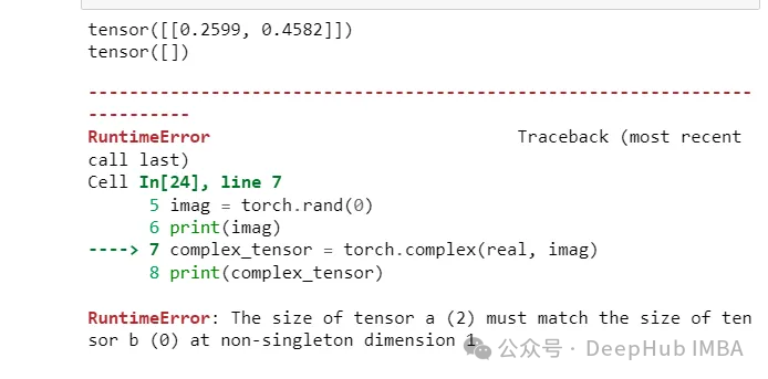
4. reshape()
reshape can change the shape of a tensor; it returns the same data as the specified array but with different specified dimension sizes.
 a = torch.tensor([1, 2, 3, 4, 5, 6, 7, 8]) print(a) print(a.reshape([4, 2]))
tensor([1, 2, 3, 4, 5, 6, 7, 8]) tensor([[1, 2],        [3, 4],        [5, 6],        [7, 8]])
If the dimensions do not match, it will raise an error.
a = torch.tensor([[1,2,3],[4,5,6]]) torch.reshape(a, (6))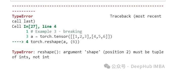
5. view()
view() is used to change the tensor in a two-dimensional format of rows and columns. We must specify the number of rows and columns.
 a=torch.FloatTensor([24, 56, 10, 20, 30,                                          40, 50, 1, 2, 3, 4, 5])
 print(a) print(a.view(4, 3))
tensor([24., 56., 10., 20., 30., 40., 50., 1., 2., 3., 4., 5.]) tensor([[24., 56., 10.],        [20., 30., 40.],        [50., 1., 2.],        [ 3., 4., 5.]])
reshape and view are both operations used to change the shape of tensors, but there are some key differences between them.
view:
-
view is a method for re-viewing a tensor.
-
It returns a new tensor that shares the same data as the original tensor, but the shape may change.
-
view operations require that the number of elements in the new shape must be the same as in the original tensor, otherwise an error will be raised.
-
view can be used to change the shape of a tensor, but only if the original tensor’s data is contiguous in memory.
reshape:
-
reshape function is also used to change the shape of a tensor.
-
Unlike view, reshape returns a new tensor that does not share the original tensor’s data. It always returns a new tensor, even if the data is contiguous in memory.
-
reshape allows changing the shape while keeping the same number of elements, as it can automatically infer the missing dimension size.
6. take()
take selects elements from a tensor according to the given indices and returns them. The input tensor is considered a one-dimensional tensor. The shape of the result matches the shape of the indices.
 a = torch.tensor([[1,2,3],                  [3, 4,7],                  [4,5,6]]) torch.take(a, torch.tensor([1,4,5]))
tensor([2, 4, 7])
If the indices exceed the length of the tensor, it will raise an error.
a = torch.tensor([[1,2,3], [3, 4,7], [4,5,6]]) torch.take(a, torch.tensor([0,3,6,8,10]))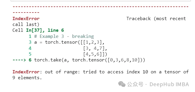
7. unbind()
unbind can be used to remove a dimension from a tensor. It returns a tuple containing all slices along the specified dimension, effectively turning the tensor into a list of tensors.
 a = torch.tensor([[1,2,3],                  [3, 4,7],                  [4,5,6]]) torch.unbind(a)
(tensor([1, 2, 3]), tensor([3, 4, 7]), tensor([4, 5, 6]))
8. reciprocal()
reciprocal returns a new tensor with the reciprocal of the input elements.
 torch.reciprocal(torch.tensor([[1.6,2.5],[3,4],[5,6]]))
tensor([[0.6250, 0.4000],        [0.3333, 0.2500],        [0.2000, 0.1667]])
9. t()
Transposing is the process of flipping the axes of a tensor. It involves swapping the rows and columns of a two-dimensional tensor or, more generally, swapping the axes of any dimensional tensor.
 E = torch.tensor([ [3, 8], [5, 6]]) F = torch.t(E) print(E) print(F)
tensor([[3, 8],        [5, 6]]) tensor([[3, 5],        [8, 6]])
10. cat()
In tensor operations, cat is the process of concatenating two or more tensors along a specified dimension to form a larger tensor. The resulting tensor has a new dimension that is the concatenation of the original dimensions of the input tensors.
 a = torch.tensor([[1, 2], [3, 4]]) b = torch.tensor([[5, 6]])
 c = torch.cat((a, b), dim=0) print(c)
tensor([[1, 2],        [3, 4],        [5, 6]])
Edited by: Yu Tengkai
Proofread by: Liang Jincheng
