Top Ten Basic Operations of TensorFlow

Click on the above “Beginner Learning Vision“, choose to add “Starred” or “Pinned“

Heavy content delivered first-hand Top Ten Basic Operations of TensorFlow

TensorFlow is an open-source, Python-based machine learning framework developed by Google. It provides interfaces in multiple programming languages such as Python, C/C++, Java, Go, and R, and has rich applications in scenarios such as image classification, audio processing, recommendation systems, and natural language processing. It is currently the most popular machine learning framework.

However, many friends have complained to me that the application of TensorFlow is too chaotic, and they feel lost while learning. Can we create a TensorFlow tutorial? Today, let’s sort out the top ten basic operations of TensorFlow together. The details are as follows:

1. TensorFlow’s Sorting and Tensors

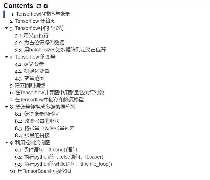
TensorFlow allows users to define tensor operations and functions as computational graphs. A tensor is a general mathematical symbol representing a multi-dimensional array that holds data values, and the dimensionality of a tensor is called its rank.

Import relevant libraries

import tensorflow as tf
import numpy as np

Get the rank of the tensor (as seen in the tf computation process in the example below)

# Get the rank of the tensor (as seen in the tf computation process in the example below)
g = tf.Graph()
# Define a computational graph
with g.as_default():
    ## Define tensors t1, t2, t3
    t1 = tf.constant(np.pi)
    t2 = tf.constant([1,2,3,4])
    t3 = tf.constant([[1,2],[3,4]])

    ## Get the rank of the tensors
    r1 = tf.rank(t1)
    r2 = tf.rank(t2)
    r3 = tf.rank(t3)

    ## Get their shapes
    s1 = t1.get_shape()
    s2 = t2.get_shape()
    s3 = t3.get_shape()
    print("shapes:",s1,s2,s3)
# Start the previously defined graph for the next operation
with tf.Session(graph=g) as sess:
    print("Ranks:",r1.eval(),r2.eval(),r3.eval())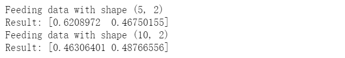

2. TensorFlow Computational Graph

The core of TensorFlow lies in constructing computational graphs and using these graphs to infer the relationships between all tensors from input to output.

Assuming there are 0-rank tensors a, b, c, to evaluate, it can be represented as the computational graph shown below:

As can be seen, the computational graph is a network of nodes, where each node acts like an operation that applies a function to the input tensor and returns zero or more tensors as output.

The steps to construct a computational graph in TensorFlow are as follows:

1. Initialize an empty computational graph

2. Add nodes (tensors and operations) to the computational graph

3. Execute the computational graph:

a. Start a new session

b. Initialize the variables in the graph

c. Run the computational graph in the session

# Initialize an empty computational graph
g = tf.Graph()
# Add nodes (tensors and operations) to the computational graph
with g.as_default():
    a = tf.constant(1,name="a")
    b = tf.constant(2,name="b")
    c = tf.constant(3,name="c")

    z = 2*(a-b)+c
    # Execute the computational graph
    ## Create a session object by calling tf.Session, which can accept a graph as a parameter (here it is g), otherwise it will start the default empty graph
    ## Use sess.run() to perform tensor operations, it will return a uniformly sized list
with tf.Session(graph=g) as sess:
    print('2*(a-b)+c =>',sess.run(z))

2*(a-b)+c => 1

3. Placeholders in TensorFlow

TensorFlow provides a special mechanism for data. One such mechanism is the use of placeholders, which are tensors with predefined types and shapes.

These tensors are added to the computational graph by calling the tf.placeholder function, and they do not include any data. However, once executing a specific node in the graph, data arrays need to be provided.

3.1 Defining Placeholders

g = tf.Graph()
with g.as_default():
    tf_a = tf.placeholder(tf.int32,shape=(),name="tf_a")  # shape=[] defines a 0-rank tensor, higher rank tensors can be represented as [n1,n2,n3], e.g., shape=(3,4,5)
    tf_b = tf.placeholder(tf.int32,shape=(),name="tf_b")
    tf_c = tf.placeholder(tf.int32,shape=(),name="tf_c")

    r1 = tf_a - tf_b
    r2 = 2*r1
    z = r2 + tf_c

3.2 Providing Data for Placeholders

When processing nodes in the graph, a Python dictionary needs to be created to provide data arrays for the placeholders.

with tf.Session(graph=g) as sess:
    feed = {
        tf_a:1,
        tf_b:2,
        tf_c:3
    }
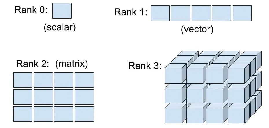
    print('z:',sess.run(z,feed_dict=feed))

z: 1

3.3 Defining Placeholders for Data Arrays with Batch Sizes

When developing neural network models, sometimes you encounter small batches of data with inconsistent sizes. One function of placeholders is to define dimensions that cannot be determined as None.

g = tf.Graph()
with g.as_default():
    tf_x = tf.placeholder(tf.float32,shape=(None,2),name="tf_x")
    x_mean = tf.reduce_mean(tf_x,axis=0,name="mean")
    np.random.seed(123)
with tf.Session(graph=g) as sess:
    x1 = np.random.uniform(low=0,high=1,size=(5,2))
    print("Feeding data with shape",x1.shape)
    print("Result:",sess.run(x_mean,feed_dict={tf_x:x1}))

    x2 = np.random.uniform(low=0,high=1,size=(10,2))
    print("Feeding data with shape",x2.shape)
    print("Result:",sess.run(x_mean,feed_dict={tf_x:x2}))

4. Variables in TensorFlow

In TensorFlow, a variable is a special type of tensor object that allows us to store and update model parameters during the training phase in the TensorFlow session.

4.1 Defining Variables

Method 1: tf.Variable() creates an object for a new variable and adds it to the computational graph.
Method 2: tf.get_variable() assumes that a variable name exists in the computational graph, it can reuse the existing value of the given variable name or create a new variable if it does not exist, so the variable name is very important!

Regardless of which method of variable definition is used, initial values are set only after calling tf.Session to start the computational graph and running the initialization operation in the session. In fact, memory is allocated for the computational graph only after initializing the TensorFlow variables.

g1 = tf.Graph()
with g1.as_default():
    w = tf.Variable(np.array([[1,2,3,4],[5,6,7,8]]),name="w")
    print(w)

4.2 Initializing Variables

Since variables are set to initial values only after calling tf.Session to start the computational graph and running the initialization operation in the session, it is crucial to initialize TensorFlow variables. This initialization process includes allocating memory space for relevant tensors and assigning initial values. The initialization methods are:

Method 1: tf.global_variables_initializer function returns to initialize all existing variables in the computational graph, note that variables must be defined before initialization, otherwise an error will be thrown!
Method 2: Store the tf.global_variables_initializer function in an init_op (name not unique, defined by yourself) object, then run it with sess.run

with tf.Session(graph=g1) as sess:
    sess.run(tf.global_variables_initializer())
    print(sess.run(w))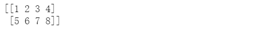

# Let's compare the relationship between defining variables and the order of initialization
g2 = tf.Graph()
with g2.as_default():
    w1 = tf.Variable(1,name="w1")
    init_op = tf.global_variables_initializer()
    w2 = tf.Variable(2,name="w2")
    with tf.Session(graph=g2) as sess:
        sess.run(init_op)
        print("w1:",sess.run(w1))

w1: 1

with tf.Session(graph=g2) as sess:
    sess.run(init_op)
    print("w2:",sess.run(w2))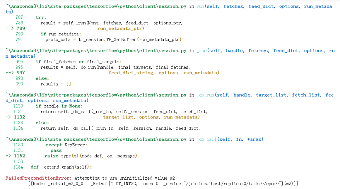

4.3 Variable Scope

Variable scope is an important concept, especially useful for building large neural network computational graphs.

You can divide the domain of variables into independent sub-parts. When creating variables, operations and tensor names created within that domain are prefixed with the domain name, and these domains can be nested.

g = tf.Graph()
with g.as_default():
    with tf.variable_scope("net_A"):   # Define a domain net_A
        with tf.variable_scope("layer-1"): # Define a sub-domain layer-1 under net_A
            w1 = tf.Variable(tf.random_normal(shape=(10,4)),name="weights")   # This variable is defined under the net_A/layer-1 domain
        with tf.variable_scope("layer-2"):
            w2 = tf.Variable(tf.random_normal(shape=(20,10)),name="weights")
    with tf.variable_scope("net_B"):   # Define a domain net_B
        with tf.variable_scope("layer-2"):
            w3 = tf.Variable(tf.random_normal(shape=(10,4)),name="weights")
    print(w1)
    print(w2)
    print(w3)

5. Building a Regression Model

The variables we need to define are:

1. Input x: placeholder tf_x
2. Input y: placeholder tf_y
3. Model parameter w: defined as variable weight
4. Model parameter b: defined as variable bias
5. Model output ̂ y^: obtained from operations

import tensorflow  as tf
import numpy as np
import matplotlib.pyplot as plt
%matplotlib inline

g = tf.Graph()
# Define computational graph
with g.as_default():
    tf.set_random_seed(123)
        ## placeholder
    tf_x = tf.placeholder(shape=(None),dtype=tf.float32,name="tf_x")
    tf_y = tf.placeholder(shape=(None),dtype=tf.float32,name="tf_y")
        ## define the variable (model parameters)
    weight = tf.Variable(tf.random_normal(shape=(1,1),stddev=0.25),name="weight")
    bias = tf.Variable(0.0,name="bias")
        ## build the model
    y_hat = tf.add(weight*tf_x,bias,name="y_hat")
        ## compute the cost
    cost = tf.reduce_mean(tf.square(tf_y-y_hat),name="cost")
        ## train the model
    optim = tf.train.GradientDescentOptimizer(learning_rate=0.001)
    train_op = optim.minimize(cost,name="train_op")

# Create a session to start the computational graph and train the model
## Create a random toy dataset for regression
np.random.seed(0)
def make_random_data():
    x = np.random.uniform(low=-2,high=4,size=100)
    y = []
    for t in x:
        r = np.random.normal(loc=0.0,scale=(0.5 + t*t/3),size=None)
        y.append(r)
    return x,1.726*x-0.84+np.array(y)

x,y = make_random_data()
plt.plot(x,y,'o')
plt.show()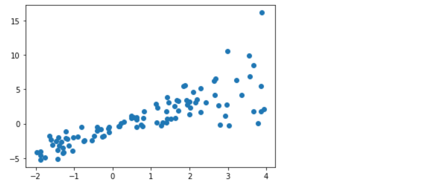

## train/test splits
x_train,y_train = x[:100],y[:100]
x_test,y_test = x[100:],y[100:]
n_epochs = 500
train_costs  = []
with tf.Session(graph=g) as sess:
    sess.run(tf.global_variables_initializer())
        ## train the model for n_epochs
    for e in range(n_epochs):
        c,_ = sess.run([cost,train_op],feed_dict={tf_x:x_train,tf_y:y_train})
        train_costs.append(c)
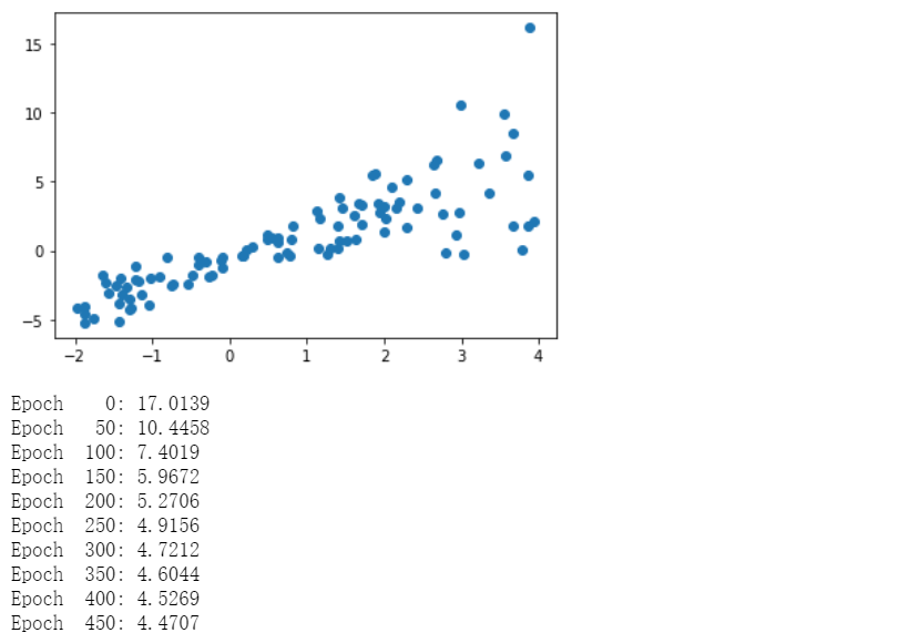
        if not e % 50:
            print("Epoch %4d: %.4f"%(e,c))
plt.plot(train_costs)
plt.show()

6. Executing Objects in TensorFlow Computational Graph with Tensor Names

Simply change

sess.run([cost,train_op],feed_dict={tf_x:x_train,tf_y:y_train})

sess.run(['cost:0','train_op:0'],feed_dict={'tf_x:0':x_train,'tf_y:0':y_train})

Note: Only tensor names have the :0 suffix, operations do not have the :0 suffix, for example, train_op does not have train_op:0

## train/test splits
x_train,y_train = x[:100],y[:100]
x_test,y_test = x[100:],y[100:]
n_epochs = 500
train_costs  = []
with tf.Session(graph=g) as sess:
    sess.run(tf.global_variables_initializer())
        ## train the model for n_epochs
    for e in range(n_epochs):
        c,_ = sess.run(['cost:0','train_op'],feed_dict={'tf_x:0':x_train,'tf_y:0':y_train})
        train_costs.append(c)
        if not e % 50:
            print("Epoch %4d: %.4f"%(e,c))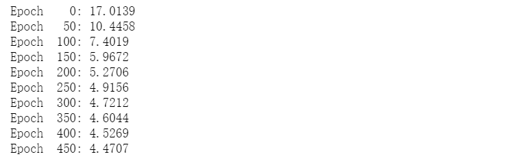

7. Saving and Restoring Models in TensorFlow

Training neural networks can take days or weeks, so we need to save the trained model for future use.

The method of saving is to add: saver = tf.train.Saver() when defining the computational graph, and after training, input saver.save(sess,’./trained-model’)

g = tf.Graph()
# Define computational graph
with g.as_default():
    tf.set_random_seed(123)
        ## placeholder
    tf_x = tf.placeholder(shape=(None),dtype=tf.float32,name="tf_x")
    tf_y = tf.placeholder(shape=(None),dtype=tf.float32,name="tf_y")
        ## define the variable (model parameters)
    weight = tf.Variable(tf.random_normal(shape=(1,1),stddev=0.25),name="weight")
    bias = tf.Variable(0.0,name="bias")
        ## build the model
    y_hat = tf.add(weight*tf_x,bias,name="y_hat")
        ## compute the cost
    cost = tf.reduce_mean(tf.square(tf_y-y_hat),name="cost")
        ## train the model
    optim = tf.train.GradientDescentOptimizer(learning_rate=0.001)
    train_op = optim.minimize(cost,name="train_op")
    saver = tf.train.Saver()
# Create a session to start the computational graph and train the model
## create a random toy dataset for regression
np.random.seed(0)
def make_random_data():
    x = np.random.uniform(low=-2,high=4,size=100)
    y = []
    for t in x:
        r = np.random.normal(loc=0.0,scale=(0.5 + t*t/3),size=None)
        y.append(r)
    return x,1.726*x-0.84+np.array(y)

x,y = make_random_data()
plt.plot(x,y,'o')
plt.show()
## train/test splits
x_train,y_train = x[:100],y[:100]
x_test,y_test = x[100:],y[100:]
n_epochs = 500
train_costs  = []
with tf.Session(graph=g) as sess:
    sess.run(tf.global_variables_initializer())
        ## train the model for n_epochs
    for e in range(n_epochs):
        c,_ = sess.run(['cost:0','train_op'],feed_dict={'tf_x:0':x_train,'tf_y:0':y_train})
        train_costs.append(c)
        if not e % 50:
            print("Epoch %4d: %.4f"%(e,c))
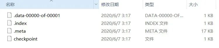
    saver.save(sess,'C:/Users/Leo/Desktop/trained-model/')

# Load the saved model
g2 = tf.Graph()
with tf.Session(graph=g2) as sess:
    new_saver = tf.train.import_meta_graph("C:/Users/Leo/Desktop/trained-model/.meta")
    new_saver.restore(sess,'C:/Users/Leo/Desktop/trained-model/')
    y_pred = sess.run('y_hat:0',feed_dict={'tf_x:0':x_test})

## Visualize the model
x_arr = np.arange(-2,4,0.1)
g2 = tf.Graph()
with tf.Session(graph=g2) as sess:
    new_saver = tf.train.import_meta_graph("C:/Users/Leo/Desktop/trained-model/.meta")
    new_saver.restore(sess,'C:/Users/Leo/Desktop/trained-model/')
    y_arr = sess.run('y_hat:0',feed_dict={'tf_x:0':x_arr})
    plt.figure()
    plt.plot(x_train,y_train,'bo')
    plt.plot(x_test,y_test,'bo',alpha=0.3)
    plt.plot(x_arr,y_arr.T[:,0],'-r',lw=3)
    plt.show()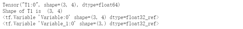

8. Converting Tensors into Multi-dimensional Data Arrays

8.1 Obtaining the Shape of a Tensor

In numpy, we can use arr.shape to obtain the shape of a Numpy array, while in TensorFlow, we use the tf.get_shape function:

Note: The result of the tf.get_shape function cannot be indexed, it needs to be converted to a list using as.list() before indexing.

g = tf.Graph()
with g.as_default():
    arr = np.array([[1.,2.,3.,3.5],[4.,5.,6.,6.5],[7.,8.,9.,9.5]])
    T1 = tf.constant(arr,name="T1")
    print(T1)
    s = T1.get_shape()
    print("Shape of T1 is ",s)
    T2 = tf.Variable(tf.random_normal(shape=s))
    print(T2)
    T3 = tf.Variable(tf.random_normal(shape=(s.as_list()[0],)))
    print(T3)

8.2 Changing the Shape of a Tensor

Now let’s see how TensorFlow changes the shape of a tensor, in Numpy we can use np.reshape or arr.reshape, and in one dimension we can use -1 to automatically calculate the last dimension. In TensorFlow, we call tf.reshape

with g.as_default():
    T4 = tf.reshape(T1,shape=[1,1,-1],name="T4")
    print(T4)
    T5 = tf.reshape(T1,shape=[1,3,-1],name="T5")
    print(T5)

with tf.Session(graph=g) as sess:
    print(sess.run(T4))
    print()
    print(sess.run(T5))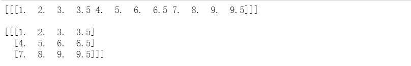

8.3 Splitting Tensors into Tensor Lists

with g.as_default():
    tf_splt = tf.split(T5,num_or_size_splits=2,axis=2,name="T8")
    print(tf_splt)

8.4 Concatenating Tensors

g = tf.Graph()
with g.as_default():
    t1 = tf.ones(shape=(5,1),dtype=tf.float32,name="t1")
    t2 = tf.zeros(shape=(5,1),dtype=tf.float32,name="t2")
    print(t1)
    print(t2)

with g.as_default():
    t3 = tf.concat([t1,t2],axis=0,name="t3")
    print(t3)
    t4 = tf.concat([t1,t2],axis=1,name="t4")
    print(t4)

with tf.Session(graph=g) as sess:
    print(t3.eval())
    print()
    print(t4.eval())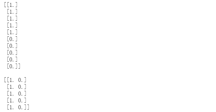

with tf.Session(graph=g) as sess:
    print(sess.run(t3))
    print()
    print(sess.run(t4))

9. Using Control Flow Graphs

This section mainly discusses executing control flow statements in TensorFlow similar to Python’s if statements, while loops, if…else statements, etc.

9.1 Conditional Statements

tf.cond() statement Let’s try it:

x,y = 1.0,2.0
g = tf.Graph()
with g.as_default():
    tf_x = tf.placeholder(dtype=tf.float32,shape=None,name="tf_x")
    tf_y = tf.placeholder(dtype=tf.float32,shape=None,name="tf_y")
    res = tf.cond(tf_x<tf_y,lambda: tf.add(tf_x,tf_y,name="result_add"),lambda: tf.subtract(tf_x,tf_y,name="result_sub"))
    print("Object:",res)  # The object is named "cond/Merge:0"
    with tf.Session(graph=g) as sess:
    print("x<y: %s -> Result:"%(x<y),res.eval(feed_dict={"tf_x:0":x,"tf_y:0":y}))
    x,y = 2.0,1.0
    print("x<y: %s -> Result:"%(x<y),res.eval(feed_dict={"tf_x:0":x,"tf_y:0":y}))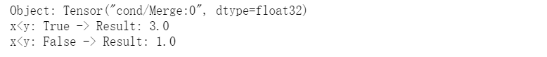

9.2 Executing Python’s if…else Statements

tf.case()

f1 = lambda: tf.constant(1)
f2 = lambda: tf.constant(0)
result = tf.case([(tf.less(x,y),f1)],default=f2)
print(result)

9.3 Executing Python’s while Statements

tf.while_loop()

i = tf.constant(0)
threshold = 100
c = lambda i: tf.less(i,100)
b = lambda i: tf.add(i,1)
r = tf.while_loop(cond=c,body=b,loop_vars=[i])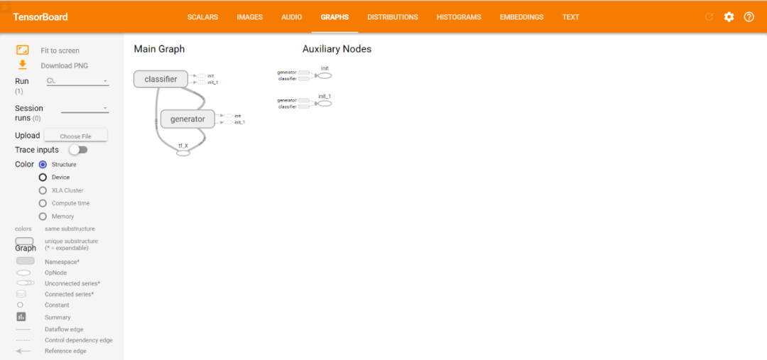
print(r)

10. Visualizing Graphs with TensorBoard

TensorBoard is a very good tool for TensorFlow, responsible for visualization and model learning. Visualization allows us to see the connections between nodes, explore their dependencies, and debug models when necessary.

def build_classifier(data, labels, n_classes=2):
    data_shape = data.get_shape().as_list()
    weights = tf.get_variable(name='weights',                              shape=(data_shape[1], n_classes),                              dtype=tf.float32)
    bias = tf.get_variable(name='bias',                           initializer=tf.zeros(shape=n_classes))
    print(weights)
    print(bias)
    logits = tf.add(tf.matmul(data, weights),                    bias,                    name='logits')
    print(logits)
    return logits, tf.nn.softmax(logits)

def build_generator(data, n_hidden):
    data_shape = data.get_shape().as_list()
    w1 = tf.Variable(        tf.random_normal(shape=(data_shape[1],                                n_hidden)),        name='w1')
    b1 = tf.Variable(tf.zeros(shape=n_hidden),                     name='b1')
    hidden = tf.add(tf.matmul(data, w1), b1,                    name='hidden_pre-activation')
    hidden = tf.nn.relu(hidden, 'hidden_activation')            
w2 = tf.Variable(        tf.random_normal(shape=(n_hidden,                                data_shape[1])),        name='w2')
    b2 = tf.Variable(tf.zeros(shape=data_shape[1]),                     name='b2')
    output = tf.add(tf.matmul(hidden, w2), b2,                    name = 'output')
    return output, tf.nn.sigmoid(output)

batch_size=64
g = tf.Graph()
with g.as_default():
    tf_X = tf.placeholder(shape=(batch_size, 100),                          dtype=tf.float32,                          name='tf_X')
    ## build the generator
    with tf.variable_scope('generator'):
        gen_out1 = build_generator(data=tf_X,                                   n_hidden=50)
        ## build the classifier
    with tf.variable_scope('classifier') as scope:
        ## classifier for the original data:
        cls_out1 = build_classifier(data=tf_X,                                    labels=tf.ones(                                        shape=batch_size))
                ## reuse the classifier for generated data
        scope.reuse_variables()
        cls_out2 = build_classifier(data=gen_out1[1],                                    labels=tf.zeros(                                        shape=batch_size))
                init_op = tf.global_variables_initializer()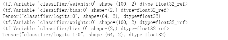

with tf.Session(graph=g) as sess:
    sess.run(tf.global_variables_initializer())
    file_writer = tf.summary.FileWriter(logdir="C:/Users/Leo/Desktop/trained-model/logs/",graph=g)

After entering cmd in win+R, enter the command:

tensorboard --logdir="C:/Users/Leo/Desktop/trained-model/logs"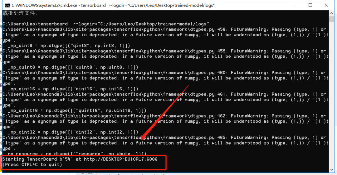

Then copy this link into the browser to open:

Download 1: OpenCV-Contrib Extension Module Chinese Tutorial

Reply in the background of the “Beginner Learning Vision” public account:Extension Module Chinese Tutorial, you can download the first OpenCV extension module tutorial in Chinese on the Internet, covering installation of extension modules, SFM algorithms, stereo vision, target tracking, biological vision, super-resolution processing and more than twenty chapters.

Download 2: Python Vision Practical Projects 52 Lectures

Reply in the background of the “Beginner Learning Vision” public account: Python Vision Practical Projects, you can download 31 vision practical projects including image segmentation, mask detection, lane line detection, vehicle counting, adding eyeliner, license plate recognition, character recognition, emotion detection, text content extraction, facial recognition, etc., to help quickly learn computer vision.

Download 3: OpenCV Practical Projects 20 Lectures

Reply in the background of the “Beginner Learning Vision” public account: OpenCV Practical Projects 20 Lectures, you can download 20 practical projects based on OpenCV, achieving advanced learning of OpenCV.

Discussion Group

Welcome to join the public account reader group to exchange with peers, currently there are WeChat groups for SLAM, three-dimensional vision, sensors, autonomous driving, computational photography, detection, segmentation, recognition, medical imaging, GAN, algorithm competitions (will gradually be subdivided in the future), please scan the following WeChat number to join the group, note: “nickname + school/company + research direction”, for example: “Zhang San + Shanghai Jiao Tong University + Visual SLAM”. Please follow the format, otherwise it will not be approved. Successful additions will be invited into the relevant WeChat groups based on research direction. Please do not send advertisements in the group, otherwise you will be asked to leave the group, thank you for your understanding~

1. TensorFlow’s Sorting and Tensors

Leave a Comment Cancel reply