
Today, instead of sharing a paper, let’s discuss some classic algorithms in machine learning.
Despite the current buzz in the capital market around embodied intelligence and large models, it is undeniable that we are still in the stage of weak artificial intelligence. Strong artificial intelligence, of course, is a vision and goal for the future development of AI.
Weak artificial intelligence has become an indispensable part of everyone’s life over the years. Next, let’s take our smartphones as an example to discuss.
The image below shows some common applications installed on a typical iPhone. Many might not guess that artificial intelligence technology is the core driving force behind many applications on smartphones.
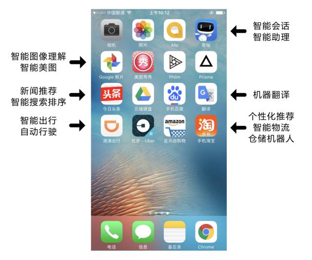
Figure 1: Relevant Applications on iPhone
Smart assistant applications like Apple’s Siri, Baidu’s DuerOS, and Microsoft’s Xiaoice are trying to revolutionize the way you interact with your phone, turning it into a smart assistant. News applications rely on intelligent recommendation technologies to push the most suitable content to you; beauty apps like MeituPic automatically perform intelligent artistic creations for recruitment and videos;
Shopping applications use intelligent logistics technologies to help companies efficiently and safely distribute goods, enhancing buyer satisfaction; Didi Chuxing helps drivers choose routes, and in the near future, autonomous driving technology will redefine smart commuting. All of this is primarily attributed to a method of achieving artificial intelligence—machine learning.
Traditional machine learning algorithms include decision trees, clustering, Bayesian classification, support vector machines, EM, Adaboost, and more.
This article will provide a commonsense introduction to commonly used algorithms without code or complex theoretical derivations, just illustrating what these algorithms are and how they are applied.
Classify based on some features, asking a question at each node to divide the data into two categories, and continuing to ask questions. These questions are learned from existing data, and when new data is input, it can be classified to the appropriate leaf based on the questions in this tree.
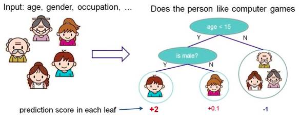
Figure 2: Schematic Diagram of Decision Tree Principles
Randomly select data from the source data to form several subsets:
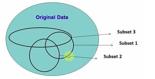
Figure 3-1: Schematic Diagram of Random Forest Principles
The S matrix is the source data, with 1-N data points; A, B, and C are features, and the last column C is the category:
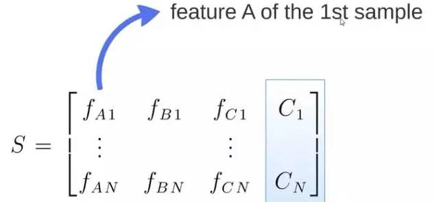
Generate M subsets randomly from S:
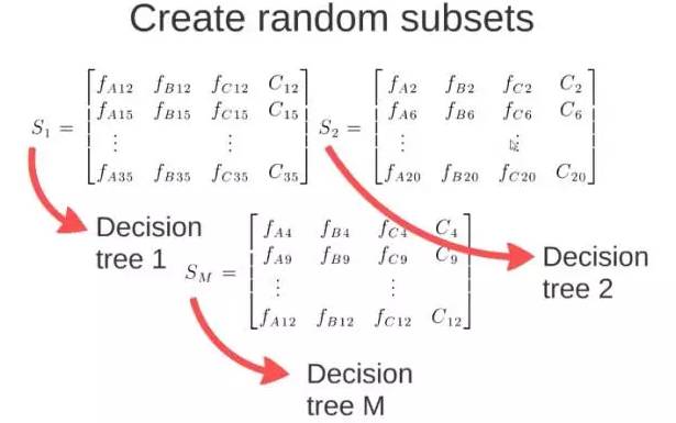
These M subsets yield M decision trees: input new data into these M trees to obtain M classification results. Count to see which class has the highest predicted count, and this class will be the final prediction result.
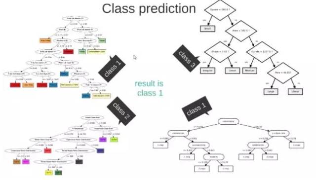
Figure 3-2: Random Forest Effect Display
When the prediction target is a probability, the range must satisfy being greater than or equal to 0 and less than or equal to 1. A pure linear model cannot achieve this because if the domain is not within a certain range, the range will exceed the specified interval.
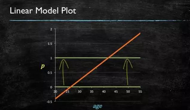
Figure 4-1: Linear Model Diagram
Therefore, a model of this shape will be better:
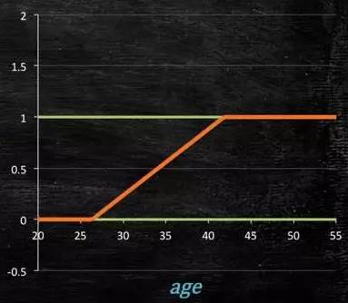
Figure 4-2
How do we obtain such a model?
This model needs to satisfy two conditions: “greater than or equal to 0” and “less than or equal to 1”. A model that is greater than or equal to 0 can use absolute values or squares; here we use the exponential function, which is always greater than 0; to ensure it is less than or equal to 1, we use division, with the numerator being itself and the denominator being itself plus 1, which will always be less than 1.
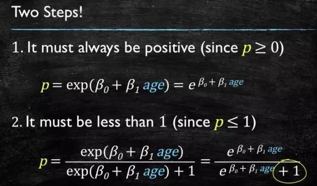
Figure 4-3
After some transformation, we obtain the logistic regression model:
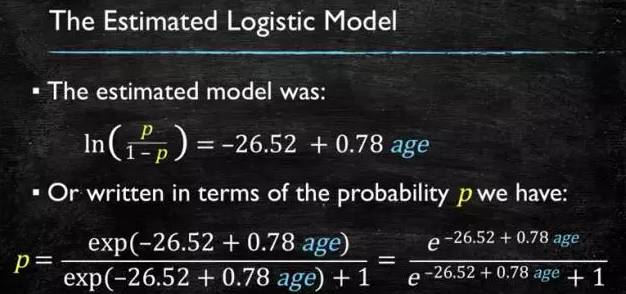
Figure 4-5
Finally, we get the logistic graph:
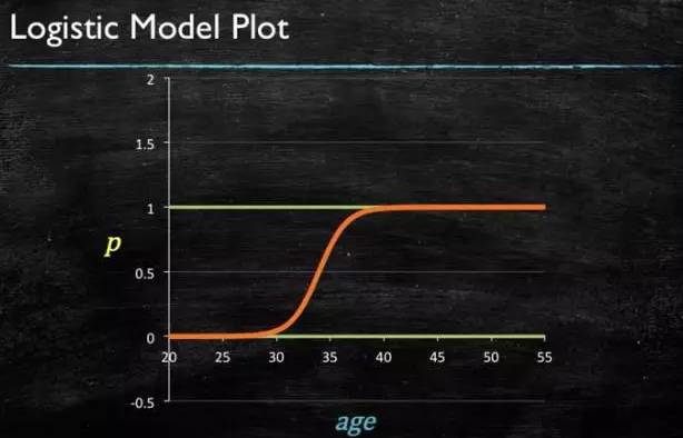
Figure 4-6: LR Model Curve Graph
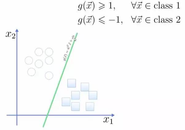
To separate two classes, we want to obtain a hyperplane, with the optimal hyperplane being the one that maximizes the margin between the two classes. The margin is the distance from the hyperplane to the nearest point, as shown in the figure. Z2 > Z1, so the green hyperplane is better.
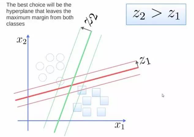
Figure 5: Classification Problem Schematic
This hyperplane can be expressed as a linear equation, where points above the line belong to one class and are greater than or equal to 1, while the other class is less than or equal to -1:
The distance from a point to the plane can be calculated using the formula in the figure:
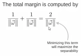
Thus, the expression for the total margin is as follows. The goal is to maximize this margin, which requires minimizing the denominator, turning it into an optimization problem:

For example, with three points, we find the optimal hyperplane, defining the weight vector as (2,3) – (1,1):
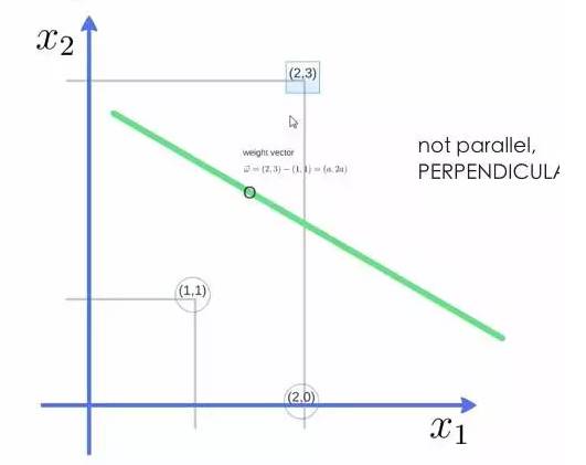
Obtaining the weight vector as (a, 2a), substituting the two points into the equation, substituting (2,3) gives a value of 1, while substituting (1,1) gives a value of -1, solving for a and the intercept w0 yields the expression for the hyperplane.
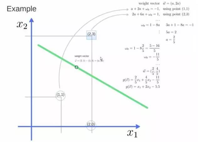
After obtaining a, substituting it into (a, 2a) gives the support vector, and substituting a and w0 into the hyperplane equation gives the support vector machine.
For example, in NLP applications: given a piece of text, return the sentiment classification, whether the attitude of this text is positive or negative:
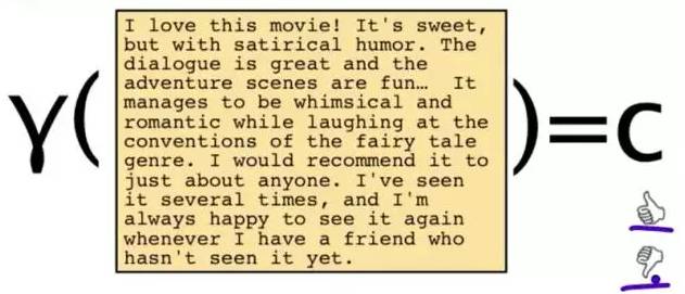
Figure 6-1: Problem Case
To solve this problem, we can only look at some of the words:
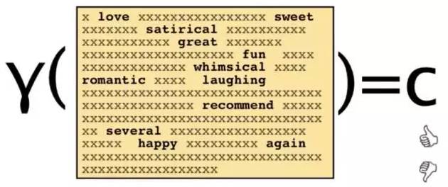
This text will be represented by some words and their counts:
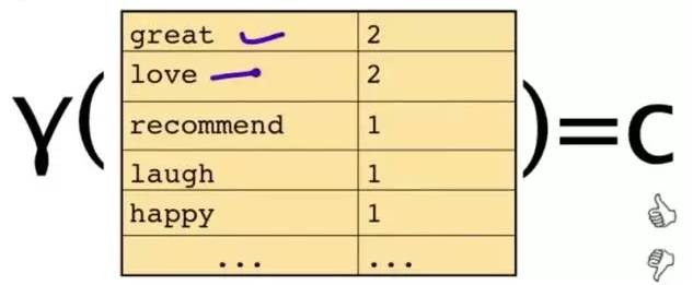
The original question is: Given a sentence, which category does it belong to? Through Bayes’ rules, this transforms into a simpler problem to solve:
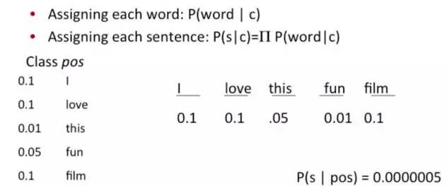
The question becomes: What is the probability of this sentence appearing in this category? Of course, do not forget the other two probabilities in the formula. For example, the probability of the word “love” appearing in the positive case is 0.1, while in the negative case it is 0.001.
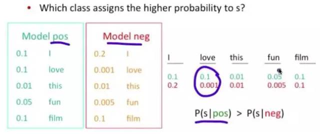
Figure 6-2: NB Algorithm Result Display
When given a new data point, the category of the data point is determined by which category is most common among the k nearest points.
For instance, to distinguish between “cats” and “dogs,” using “claws” and “sound” as features, if the circular and triangular shapes are known categories, then which category does this “star” represent?
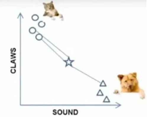
Figure 7-1: Problem Case
When k=3, the three points connected by the lines are the nearest three points. Since there are more circles, this star belongs to the category of cats.

Figure 7-2: Algorithm Steps Display
First, we need to divide a set of data into three categories: pink has a high value, yellow has a low value. Initially, we select the simplest values 3, 2, and 1 as the initial values for each category. For the remaining data, each is compared with the three initial values to calculate the distance and classify it into the category of the nearest initial value.
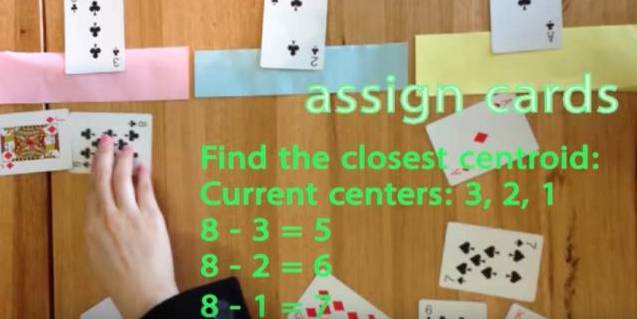
Figure 8-1: Problem Case
After categorization, calculate the average value of each category to serve as the new center point for the next round:
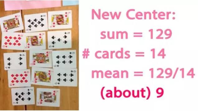
Figure 8-2
After several rounds, if the grouping no longer changes, we can stop:
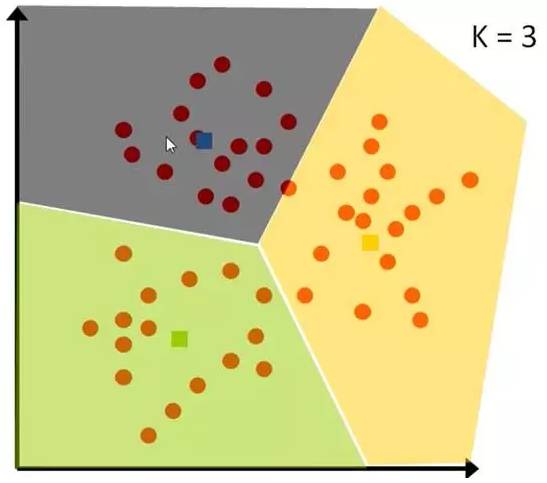

Figure 8-3: Algorithm Result Display
Adaboost is one of the methods of Boosting. Boosting combines several classifiers that do not perform well individually to create a more effective classifier.
In the image below, the two decision trees on the left and right do not perform well individually, but when the same data is input and the results are combined, the credibility increases.
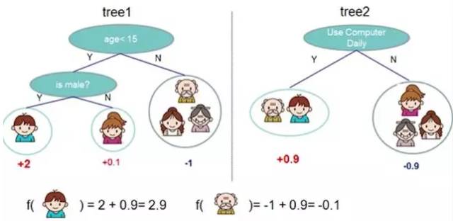
Figure 9-1: Algorithm Principle Display
An example of Adaboost in handwritten recognition involves capturing many features, such as the direction of the starting point, the distance between the start and end points, etc.
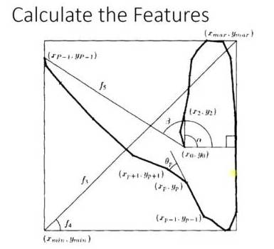
Figure 9-2
During training, the weight of each feature is determined. For instance, if the features of 2 and 3 are very similar, their weight will be small, indicating they contribute little to classification.

Figure 9-3
However, this angle alpha is highly distinctive, leading to a larger weight for this feature. The final prediction result is a comprehensive consideration of these feature results.
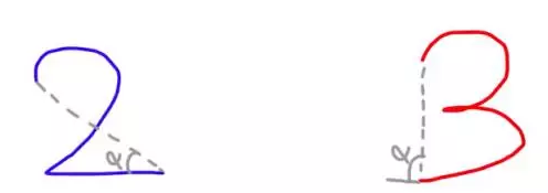
Figure 9-4
Neural Networks are suitable for inputs that may fall into at least two categories: NN consists of several layers of neurons and their connections. The first layer is the input layer, and the last layer is the output layer. Both the hidden layer and output layer have their own classifiers.
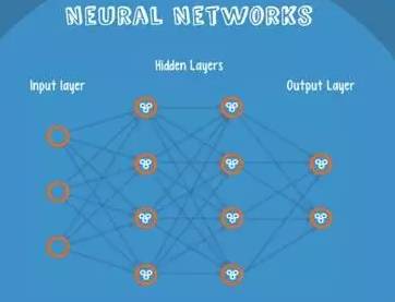
Figure 10-1: Neural Network Structure
The input is passed into the network, activated, and the computed scores are transmitted to the next layer, activating the subsequent neural layers. Finally, the scores on the output layer nodes represent scores belonging to each class. In the example below, the classification result is class 1. The same input is transmitted to different nodes, resulting in different outcomes due to varying weights and biases at each node, which is known as forward propagation.
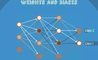
Figure 10-2: Algorithm Result Display
Markov Chains consist of states and transitions. For example, based on the sentence ‘the quick brown fox jumps over the lazy dog’, we want to obtain Markov chains.
The steps involve assigning each word as a state and then calculating the probabilities of transitions between states.
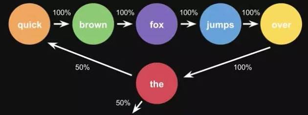
Figure 11-1: Markov Principle Diagram
This is the probability calculated from one sentence. When you do statistics with a large volume of text, you will get a larger state transition matrix, for example, the words that can follow ‘the’ and their corresponding probabilities.
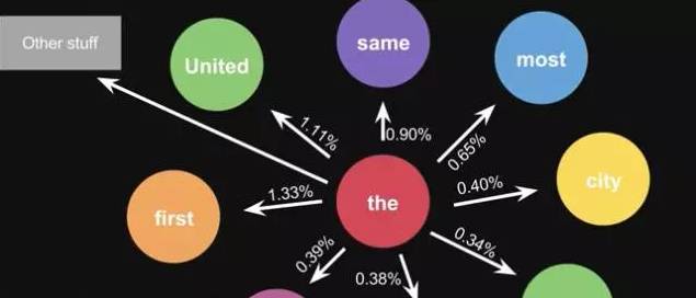
Figure 11-2: Algorithm Result Display
The above ten types of machine learning algorithms are practitioners of artificial intelligence development, widely used in data mining and small sample AI problems even today.
Deep Blue Academy: An online education platform for cutting-edge technologies like artificial intelligence.

The key is whether it can solve the students’ problems.