MLNLP community is a well-known machine learning and natural language processing community both domestically and internationally, with an audience covering NLP graduate students, university professors, and industry researchers.

The Vision of the Community is to promote communication and progress between the academic and industrial circles of natural language processing and machine learning, especially for beginners.

Reprinted from | Jishi Platform

Author丨Tech Beast

TL;DR

This article explores a new class of diffusion models based on Transformers called Diffusion Transformers (DiTs). The article replaces the commonly used UNet architecture with a Transformer architecture when training latent diffusion models, with the Transformer operating on latent patches.

The author explores the scalability of DiT, finding that DiT models with higher GFLOPs consistently achieve better FID values by increasing the width or depth of the Transformer or the number of input tokens. The largest DiT-XL/2 model outperforms all previous diffusion models in tests on ImageNet 512×512 and 256×256, achieving an FID value of 2.27.

What This Article Does

1. Explores a new class of Transformer-based diffusion models called Diffusion Transformers (DiTs).
2. Studies the scalability of DiT in terms of model complexity (GFLOPs) and sample quality (FID).
3. Proves that the U-Net architecture in diffusion models can be replaced by Transformers using the Latent Diffusion Models (LDMs) framework.

DiT: Building Diffusion Models with Transformers

Paper Title: Scalable Diffusion Models with Transformers (ICCV 2023, Oral)

Paper URL:

https//arxiv.org/pdf/2212.09748.pdf

Paper Homepage:

https//www.wpeebles.com/DiT.html

• 1 DiT Paper Interpretation:

1.1 Introducing Transformers into Diffusion Models

Machine learning is experiencing a renaissance brought by the Transformer architecture: many fields such as NLP and CV are being covered by Transformer models. Although Transformers are widely used in autoregressive models, this architecture has been less adopted in generative models. For instance, the classic method for generative models in the image domain, Diffusion Models, has always used convolution-based U-Net architectures as the backbone.

The pioneering work of Diffusion Models, DDPM, first introduced diffusion models based on U-Net backbone networks. U-Net inherits from PixelCNN++, with minimal changes. Compared to standard U-Net, additional spatial self-attention blocks (an essential component in Transformers) are interspersed at lower resolutions. This work explores several architectural choices for U-Net, such as adaptive normalization layers that inject conditional information and channel counts into convolutional layers. However, the high-level design of U-Net in DDPM largely remains unchanged.

The purpose of this article is to explore the importance of architectural choices in Diffusion Models and provide a baseline for future research in generative models. The conclusion of this article indicates that the design of U-Net architecture is not crucial for the performance of Diffusion Models, and they can easily be replaced by Transformers.

This article demonstrates that Diffusion Models can also benefit from the Transformer architecture, taking advantage of its training schemes, scalability, robustness, efficiency, and more. Standardized architectures will also open new possibilities for cross-domain research.

1.2 Introduction to Diffusion Models

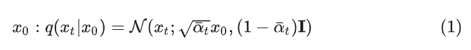
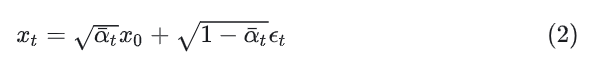
DDPM

The Gaussian diffusion model assumes a forward noising process, during which noise is gradually applied to real data:

Where the constant is a hyperparameter. By using the reparameterization trick, the above can be simplified to:

In which, .

The reparameterization trick rewrites a random variable as a deterministic function of a noise variable, allowing this non-random variable to be optimized through gradient descent. For example, if there is a , then can be rewritten as:

Thus, the 2nd equation holds.

The Diffusion Model learns a reverse process: given the current step’s image , predicts the previous step’s image through network parameters .

This optimization target function is quite complex, and the conclusion derived through the variational lower bound method is to optimize the following equation (detailed derivation can be referenced in the pioneering work DDPM):

Since both and are Gaussian, can be evaluated using the means and covariances of the two distributions.

During training, the diffusion model uses predicted noise and GT noise values for training. The author uses to train , and uses to train . Once the diffusion model is trained, new images can be sampled, and then sampled step by step through the Reparameterization trick.

Latent Diffusion Models

Training the Diffusion Model directly in high-resolution pixel space leads to massive computational costs. LDM solves this issue through a two-stage method:

1. Learn an AutoEncoder to compress images into a smaller spatial representation.
2. Train a diffusion model on instead of the original image, during which is frozen.
3. When generating new images, sample from the diffusion model, then decode back to images using the learned decoder.

1.3 Introduction to DiT Architecture

1.3.1 Patchify Process

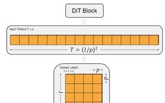
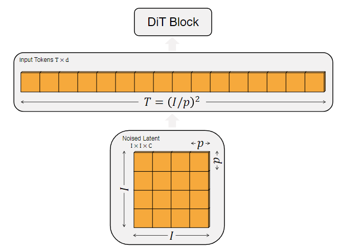
For an image of , the dimensions are . The first step of DiT is the same as ViT, which is to Patchify the image and pass it through Linear Embedding, ultimately transforming it into tokens of dimension . After Patchifying, the author applies standard ViT frequency positional encoding (sine-cosine version) to all input tokens.

The number of tokens is determined by the patch size. As shown in Figure 1, the relationship between patch size and the number of tokens satisfies . As the patch size decreases, the number of tokens increases. Halving will quadruple , resulting in a fourfold increase in computational load. Although this significantly impacts GFLOPs, it does not substantially affect the number of parameters.

The author uses in the DiT design space.

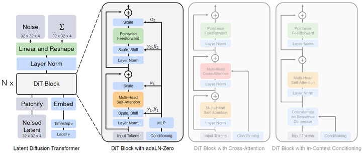
1.3.2 DiT Block Design

After Patchifying, the input tokens begin to enter a series of Transformer Blocks. Besides the noisy image input, the Diffusion Model sometimes processes additional conditional information, such as noise time step ttt, class labels ccc, and natural language.

The author explores four different types of Transformer Blocks to handle conditional inputs in different ways. These designs involve minor modifications to the standard ViT Block, and all Block designs are illustrated in Figure 2.

• In-Context Conditioning

In cases with conditional inputs like this, the In-context conditioning method simply requires adding the time step and class labels as two additional tokens to the input sequence. The author treats them as indistinguishable from the image tokens. This is somewhat similar to the [CLS] token in ViT. This allows DiT to use the standard ViT Block without any modifications. After the last Block, the conditional tokens can be removed. The additional GFLOPs brought by this method are negligible.

• Cross-Attention Block

The method for the Cross-attention block is to concatenate the embeddings of and into a sequence of length 2, separate from the image token sequence. This operation adds a Cross-Attention block to the Transformer Block, incurring an additional GFLOPs cost of about .

• Adaptive Layer Norm (adaLN) Block

The Adaptive Layer Norm (adaLN) Block follows the adaptive normalization layer in GANs, aiming to explore its utility in diffusion models. The author does not directly learn the scaling and shifting parameters and instead derives them from the noise time step and class labels. The additional GFLOPs brought by adaLN are minimal.

• adaLN-Zero Block

Previous work has found that in supervised learning, zero-initializing the scaling factor of the first Batch Norm operation for each Block can accelerate large-scale training. The U-Net based diffusion model uses a similar initialization strategy, zero-initializing the first convolution for each Block. The author makes some improvements: in addition to regressing the scaling and shifting parameters, they also regress the scaling coefficients. The author initializes the MLP to output scaling coefficients of zero, thus initializing the DiT Block to be an Identity Function. The additional GFLOPs brought by adaLN-Zero Block can be neglected.

The author includes the above methods of In-Context Conditioning, Cross-Attention Block, Adaptive Layer Norm (adaLN) Block, adaLN-Zero Block in the design space of DiT.

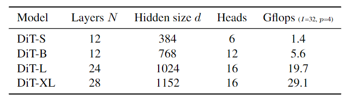
1.3.3 Model Size

Following ViT’s approach, the author considers scaling DiT from several dimensions: depth , hidden dimension , and number of heads. The author designs four different sizes of DiT models: DiT-S, DiT-B, DiT-L, and DiT-XL, ranging from 0.3 to 118.6 GFLOPs, with detailed information shown in Figure 3.

The author includes the above configurations in the design space of DiT.

1.3.4 Transformer Decoder

After the last DiT Block, the sequence of image tokens needs to be decoded into the predicted outputs of noise and the diagonal covariance matrix.

Moreover, both outputs have shapes consistent with the original spatial input. The author uses a standard linear decoder in this step, linearly decoding each token into a tensor of dimensions , where is the number of channels from the spatial input to DiT. Finally, the decoded tokens are rearranged to their original spatial layout to obtain the predicted noise and covariance.

Ultimately, the complete design space of DiT is the patch size, the architecture of DiT Block, and model size.

1.4 DiT Training Strategy

1.4.1 Training Recipe

The author trained a class-conditional latent DiT model on the ImageNet dataset, using standard experimental settings.

The resolution is set to .

Zero Initialization is used for the final Linear Layer, while others use standard weight initialization schemes from ViT. The optimizer used is AdamW, with a fixed learning rate, Batch Size of 256, and no weight decay.

Data augmentation techniques only use horizontal flips.

The author finds that learning rate warmup and regularization are not necessary for training the DiT model.

The author uses exponential moving average (EMA) with a parameter of 0.9999.

Training hyperparameters mainly come from ADM, without tuning learning rates, decay/warm-up schedules, Adam parameters, or weight decay.

1.4.2 Diffusion Model Configuration

For other components of DiT, the author uses a pre-trained Variational AutoEncoder (VAE) model from Stable Diffusion. The VAE Encoder downsampling rate is 8: Given the input image , the resulting encoding size is .

After sampling a new latent result from the diffusion model, the author uses the VAE decoder to decode it back to pixel: .

The author retains the hyperparameters used in ADM.

1.5 Exploration Process of DiT

1.5.1 DiT Architecture Design

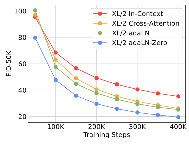
The author first explores the comparison of different conditioning strategies. For a DiT-XL/2 model, its computational complexities are: in-context (119.4 Gflops), cross-attention (137.6 Gflops), adaptive layer norm (adaLN, 118.6 Gflops), adaLN-zero (118.6 Gflops). The experimental results are shown in Figure 4.

The adaLN-Zero Block architecture achieves the lowest FID results while also being the most computationally efficient. In 400K training iterations, the FID obtained by the adaLN-Zero Block architecture is almost half that of In-Context, indicating that the conditioning strategy significantly affects the model’s quality.

Initialization is also crucial: the adaLN-Zero Block architecture performs as an identity mapping at initialization, greatly outperforming the adaLN Block architecture.

Therefore, in subsequent experiments, DiT will consistently use the adaLN-Zero Block architecture.

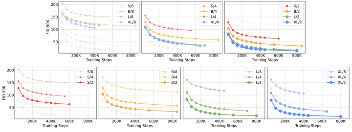
1.5.2 Scaling Model Size and Patch Size

The author trained 12 DiT models (sizes S, B, L, XL, Patch Sizes of 8, 4, 2). The following figure shows the sizes of different DiT models and their FID-50K performance. As shown in Figure 5, the GFLOPs of different sized DiT models and their FID values in 400K training iterations can be observed. It can be found that increasing model size or decreasing Batch Size can significantly improve DiT performance.

In the upper part of Figure 6, the change in FID when increasing model size while keeping patch size constant can be observed. As the model becomes deeper and wider, FID decreases.

The lower part shows the change in FID when decreasing patch size while keeping model size constant. A significant improvement in FID is observed as patch size decreases.

1.5.3 GFLOPs are Crucial for Performance

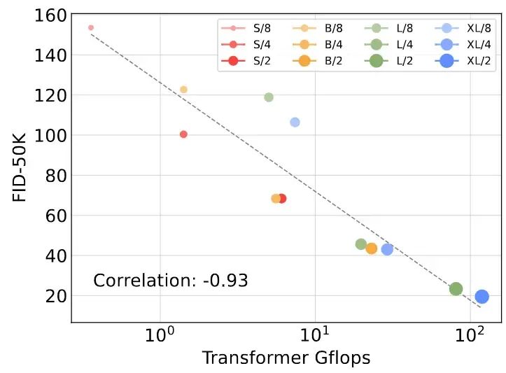
The results in Figure 5 indicate that the number of parameters alone does not determine the quality of DiT models. As the patch size decreases, the number of parameters only slightly decreases, while GFLOPs significantly increase. These results demonstrate that the GFLOPs of scaling the model is the key to performance improvement. To verify this, the author plots the FID-50K results of different GFLOPs models at 400K training steps in Figure 6. These results show that when the total GFLOPs of different DiT models are similar, their FID values are also similar, such as DiT-S/2 and DiT-B/4.

The author also finds a strong negative correlation between the GFLOPs of DiT models and FID-50K.

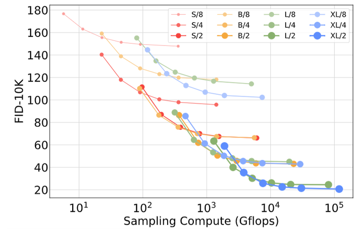
1.5.4 Larger Models are More Computationally Efficient

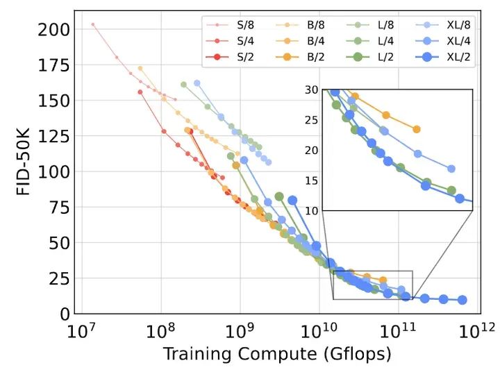
In Figure 7, the author plots the FID of all DiT models as a function of training computational resources. Training computational resources = GFLOPs – Batch Size – Training Steps 3. Here, 3 roughly considers that the computational cost of backpropagation is twice that of forward propagation.

The author finds that smaller DiT models, even with longer training times, become less computationally efficient compared to larger DiT models with fewer training steps. Furthermore, models of the same size but different patch sizes perform differently even with equivalent training computational resources. For example, at GFLOPs, XL/4 performs worse than XL/2.

In summary: larger models are more computationally efficient, and models with smaller patch sizes are more computationally efficient.

1.5.5 Visualization of Scaling Results

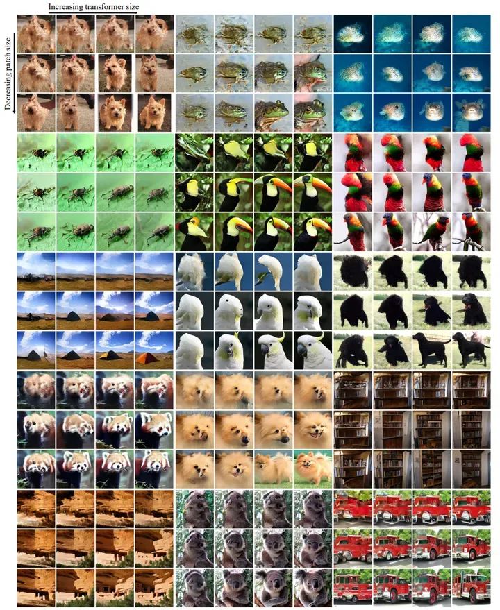
The author samples from 12 DiT models at the same starting noise, sampling noise, and class labels during training steps, as shown in Figure 8. This allows for a visual comparison of how scaling affects the quality of DiT generated samples. In fact, scaling the model size and the number of tokens can significantly improve the visual quality of the results.

1.6 DiT Experimental Results

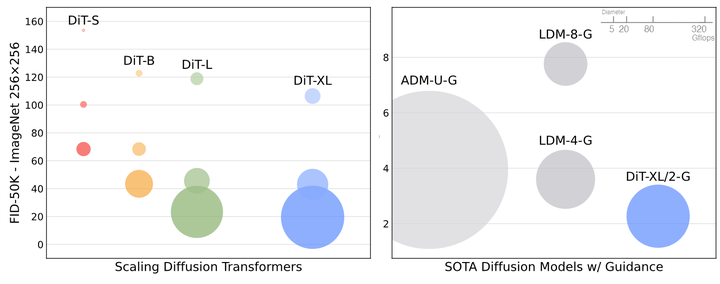
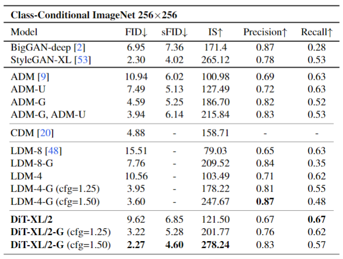
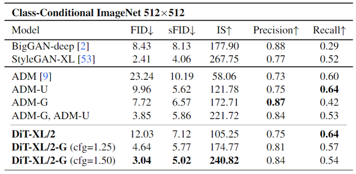
The author compares DiT with state-of-the-art generative models, with results shown in Figure 9. DiT-XL/2 outperforms all previous diffusion models, reducing the previous best FID-50K achieved by LDM to 2.27. The right side of Figure 5 shows that DiT-XL/2 (118.6 GFLOPs) is highly efficient compared to Latent Space U-Net models like LDM-4 (103.6 GFLOPs) and more efficient than Pixel Space U-Net models such as ADM (1120 GFLOPs) or ADM-U (742 GFLOPs).

The author trained a new DiT-XL/2 on ImageNet with a resolution of 512×512, 3M training iterations, and the same hyperparameters as the 256×256 model. This model’s latent dimension is 64×64×4, and the patch size is 2, resulting in 1024 tokens for the Transformer model to process. The comparison results are shown in Figure 10. DiT-XL/2 once again outperforms all previous diffusion models at this resolution, improving the previous best FID achieved by ADM from 3.85 to 3.04. Even with an increased number of tokens, DiT-XL/2 remains highly efficient, using only 524.6 GFLOPs compared to ADM’s 1983 GFLOPs and ADM-U’s 2813 GFLOPs.

Scaling Model Size or Sampling Count?

A unique aspect of Diffusion Models is that they can utilize additional computation during training by increasing the number of sampling steps when generating images. This means that the computational load of diffusion models can come from both scaling the model itself and from increasing the number of sampling steps. Therefore, the author investigates whether smaller DiT models can outperform larger models by using more sampling computations.

The author calculates the FID values of all 12 DiT models at 400K training iterations, with each image using [16, 32, 64, 128, 256, 1000] sampling steps.

The experimental results are shown in Figure 11, considering DiT-L/2 with 1000 sampling steps versus DiT-XL/2 with 128 steps. In this case:

• DiT-L/2 uses 80.7 TFLOPs to sample each image.
• DiT-XL/2 uses 15.2 TFLOPs to sample each image.

However, DiT-XL/2 still achieves better FID-10K results, indicating that increasing the sampling computational load cannot compensate for the lack of computational load from the model itself.

References

1. High-Resolution Image Synthesis with Latent Diffusion Models
2. Language Models are Few-Shot Learners
3. Generative Pretraining From Pixels
4. Zero-Shot Text-to-Image Generation
5. Language Models are Unsupervised Multitask Learners
6. Hierarchical Text-Conditional Image Generation with CLIP Latents
7. Diffusion Models Beat GANs on Image Synthesis
8. Denoising Diffusion Probabilistic Models.
9. PixelCNN++: Improving the PixelCNN with Discretized Logistic Mixture Likelihood and Other Modifications
10. Conditional Image Generation with PixelCNN Decoders
11. U-Net: Convolutional Networks for Biomedical Image Segmentation
12. Diffusion Models Beat GANs on Image Synthesis
13. FiLM: Visual Reasoning with a General Conditioning Layer
14. https://arxiv.org/pdf/2208.11970.pdf
15. A Style-Based Generator Architecture for Generative Adversarial Networks
16. Accurate, Large Minibatch SGD: Training ImageNet in 1 Hour

Technical Exchange Group Invitation

△Long press to add assistant

Scan the QR code to add the assistant’s WeChat

Please note: Name – School/Company – Research Direction

(e.g., Xiao Zhang – Harbin Institute of Technology – Dialogue System)

to apply to join technical exchange groups such as Natural Language Processing/Pytorch.

About Us

MLNLP Community is a grassroots academic community jointly built by scholars in machine learning and natural language processing from China and abroad. It has developed into a well-known community in machine learning and natural language processing, aiming to promote progress between academia, industry, and enthusiasts.

The community can provide an open exchange platform for related practitioners’ further education, employment, and research. Everyone is welcome to follow and join us.