The Ultimate Illustrated Guide to Micro Neural Networks – Multi-Layer Perceptron

Have you noticed that neural networks are everywhere? They appear in the news, in your phone, and even on your social media. But honestly, most of us don’t know how they work. Those fancy math and strange terms like “backpropagation”?

In this article, we explore the Multi-Layer Perceptron (MLP) – the most basic type of neural network – using a small network with just a few data points to classify a simple 2D dataset.

We will break down the process and illustrate each step, showing you the vibrant mathematical knowledge, how numbers and equations flow through the network, and how learning actually happens!

Definition

A Multi-Layer Perceptron (MLP) is a type of neural network that uses multiple layers of connected nodes to learn patterns. It is named for having multiple layers – typically, an input layer, one or more intermediate (hidden) layers, and an output layer.

Each node is connected to every node in the next layer. As the network learns, it adjusts the strength of these connections based on training examples. For instance, if certain connections lead to correct predictions, they become stronger. If they lead to errors, they become weaker.

This way of learning through examples helps the network recognize patterns and make predictions about new situations it has never seen before.

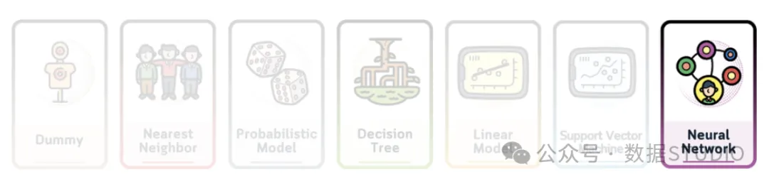
MLPs are considered fundamental in the field of neural networks and deep learning because they can handle complex problems that simple methods struggle with.

Dataset Used

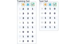
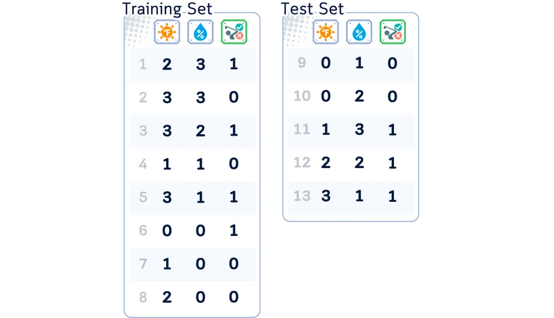
To understand how MLP works, let’s start with a simple example: a mini 2D dataset with only a few samples. We will use the same dataset from the previous article to keep things manageable.

We don’t need to train directly, but rather try to understand the key components that make up the neural network and how they work together.

Step 0: Network Structure

First, let’s look at the different parts of the network:

Nodes (Neurons)

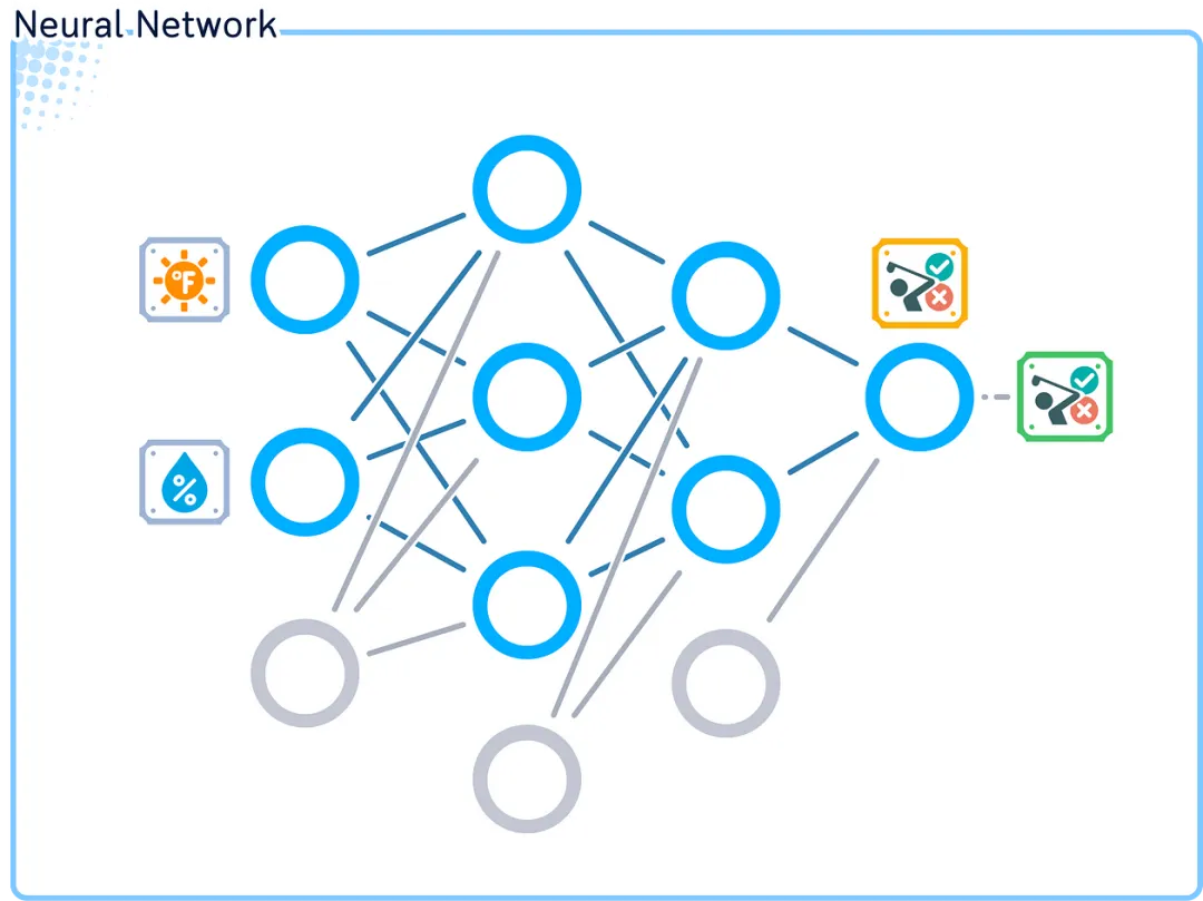
We start with the basic structure of the neural network, which consists of many individual units called nodes or neurons.

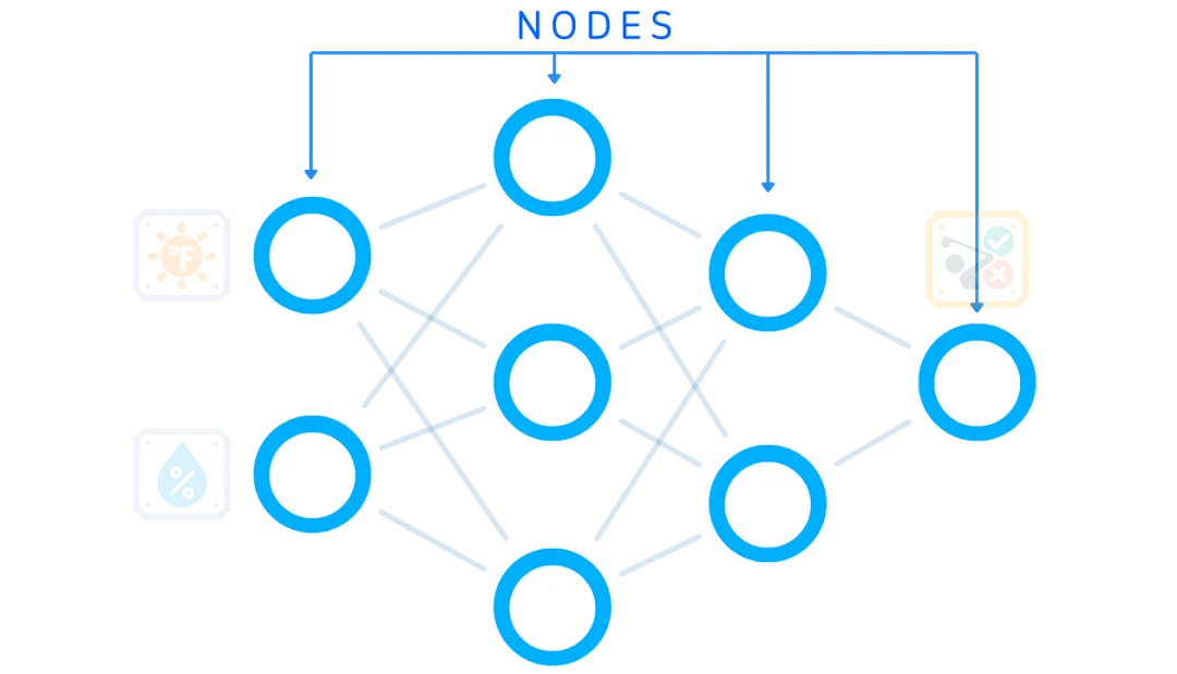
These nodes are organized into groups called layers to work together.

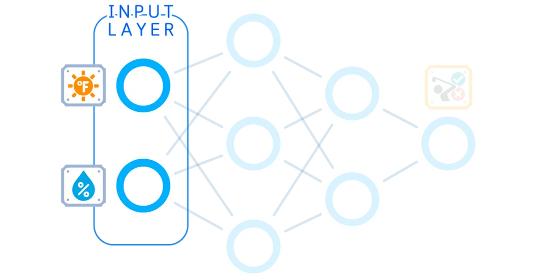
Input Layer

The input layer is our starting point. It receives our raw data, and the number of nodes here matches the number of features we have.

Hidden Layers

Next are the hidden layers. We can have one or more of these layers and choose how many nodes each layer has. Typically, as the number of layers increases, the number of nodes we use in each layer decreases.

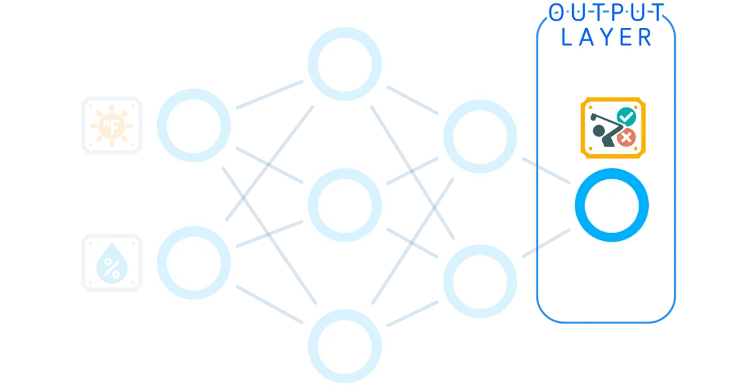
Output Layer

The final layer provides the final answer. The number of nodes in the output layer depends on our task: for binary classification or regression, we might have only one output node, while for multi-class problems, there is one node for each class.

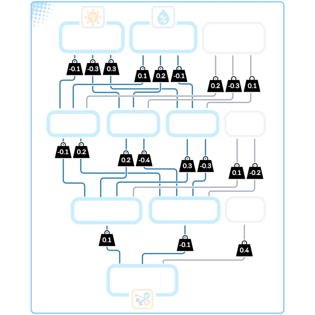
Weights

The nodes are interconnected by weights – numbers that control the importance of each piece of information. Each connection between nodes has its own weight. This means we need a lot of weights: each node in one layer connects to every node in the next layer.

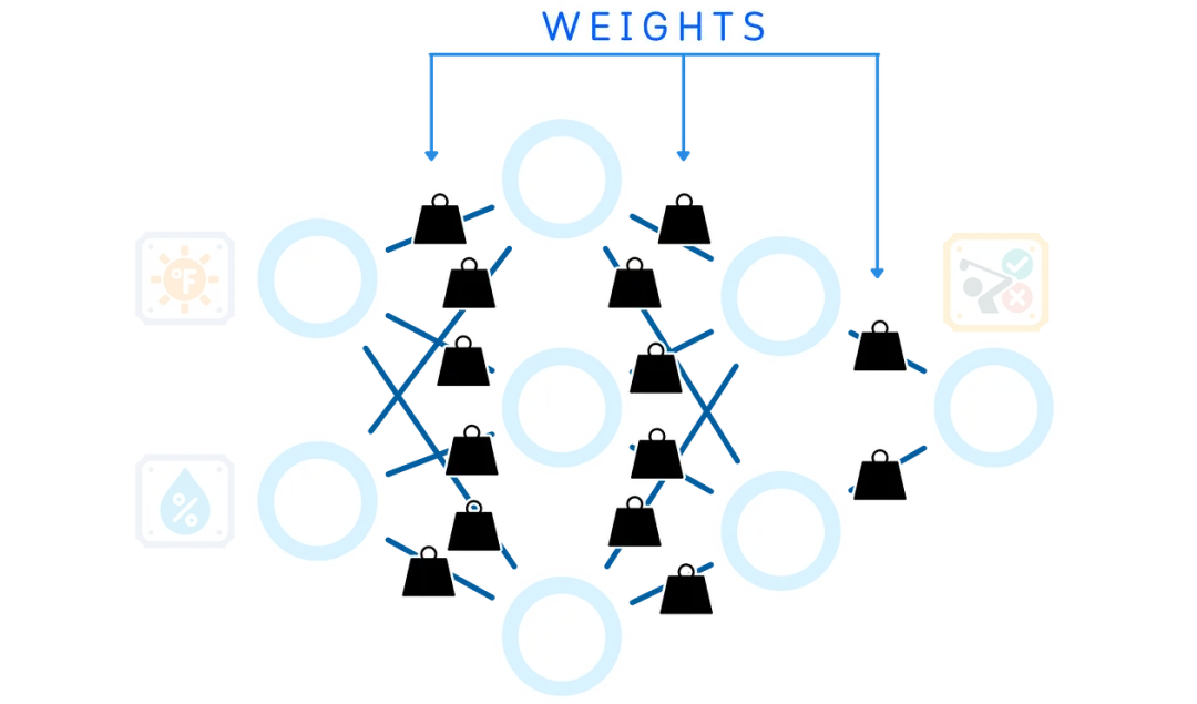
This neural network has a total of 14 weights.

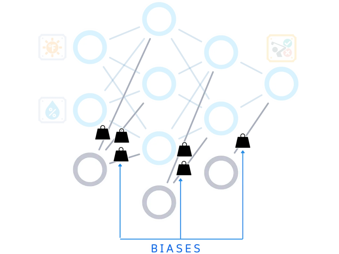
Biases

In addition to weights, each node has a bias – an extra number that helps it make better decisions. Weights control the connections between nodes, while biases help each node adjust its output.

Neural Network

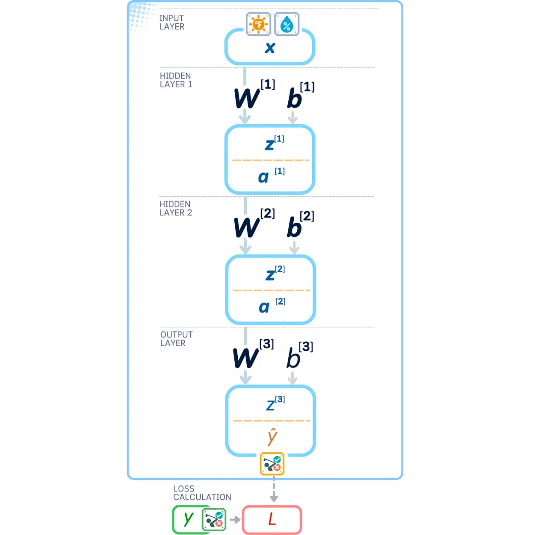
In summary, we will use and train this neural network:

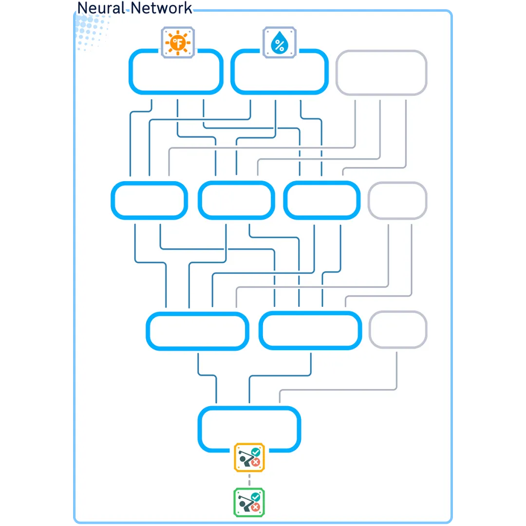
Our network consists of 4 layers: 1 input layer (2 nodes), 2 hidden layers (3 nodes and 2 nodes), and 1 output layer (1 node). This creates a 2–3–2–1 architecture.

Take a look at this new diagram that shows our network from top to bottom. I’ve updated it to make the math easier to understand: information starts at the top node, flows through each layer, and reaches the final answer at the bottom.

Now that we understand how the network is constructed, let’s look at how information propagates through the network. This is called forward propagation.

Step 1: Forward Propagation

Next, we will take a step-by-step look at how our network transforms input into output:

Weight Initialization

Before our network starts learning, we need to assign a starting value for each weight. We choose small random numbers between -1 and 1. Starting with random numbers helps our network learn without any early preferences or patterns.

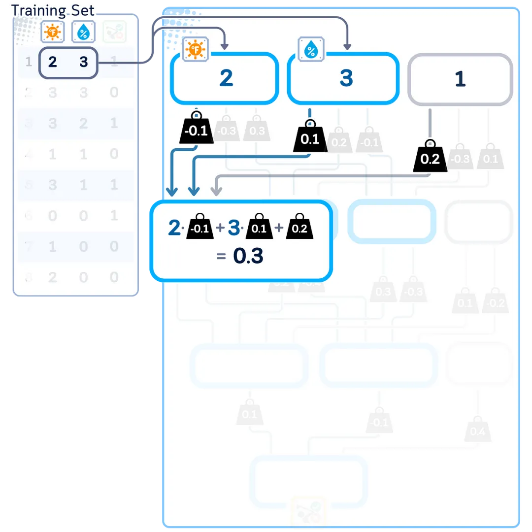
Weighted Sum

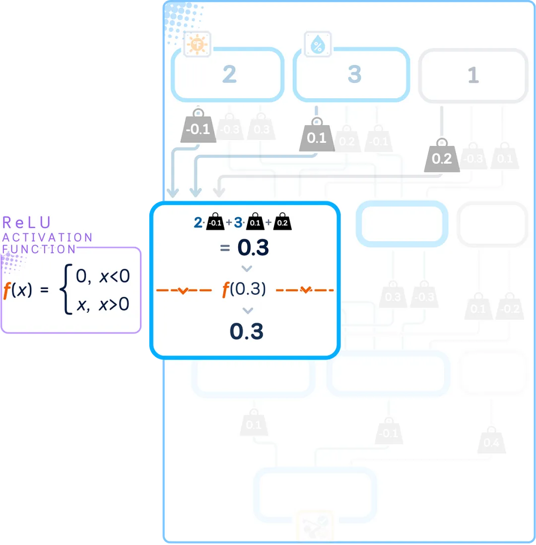
Each node processes incoming data in two steps. First, it multiplies each input by its weight and sums all these numbers. Then, it adds another number (the bias) to complete the calculation. The bias is essentially a weight with an input of constant 1.

Activation Function

Each node takes its weighted sum and runs it through an activation function to produce its output. The activation function helps our network learn complex patterns by introducing non-linear behavior.

In the hidden layers, we use the ReLU function (Rectified Linear Unit). ReLU is simple: if the number is positive, it remains unchanged; if the number is negative, it becomes zero.

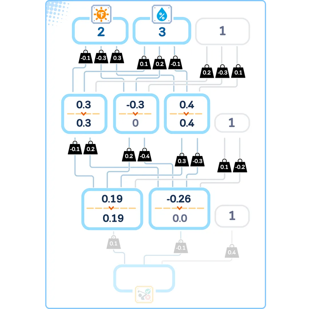
Layer-wise Calculation

This two-step process (weighted sum and activation) occurs sequentially in each layer. The computations of each layer help gradually transform our input data into the final prediction.

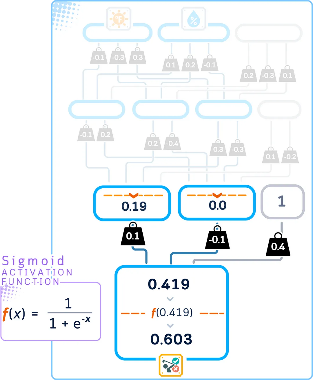
Output Generation

The last layer creates the final answer of our network. For our yes/no classification task, we use a special activation function called sigmoid in this layer.

The sigmoid function converts any number into a value between 0 and 1. This makes it very suitable for yes/no decisions because we can interpret the output as a probability: the closer to 1 indicates more likely to be “yes,” and the closer to 0 indicates more likely to be “no.”

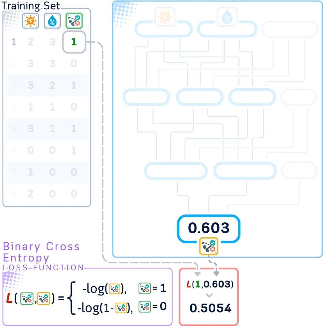
This forward propagation process transforms our input into predictions between 0 and 1. But how accurate are these predictions? Next, we will measure how close our predictions are to the correct answers.

Step 2: Loss Calculation

Loss Function

To check how our network performs, we measure the difference between its predictions and the correct answers. For binary classification, we use a method called binary cross-entropy, which shows the deviation of our predictions from the true values.

Mathematical Notation in Neural Networks

To improve the network’s performance, we need to use some mathematical notations. Before proceeding, let’s define what each symbol means:

Weights and Biases are represented as matrices, and biases as vectors (or one-dimensional matrices). The parentheses [1] indicate the layer number.

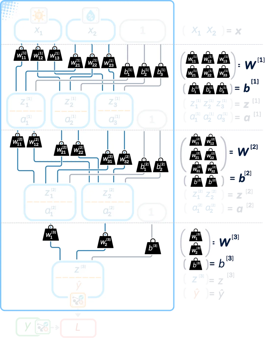
Input, Output, Weighted Sum, and Activated Values can be represented as vectors within a consistent mathematical framework.

These mathematical symbols help us accurately write down what our network is doing:

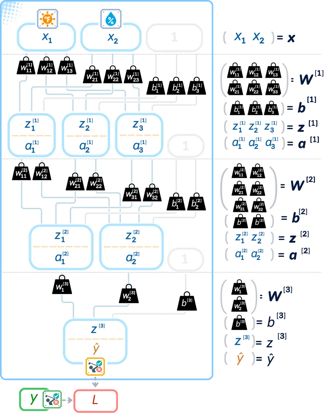
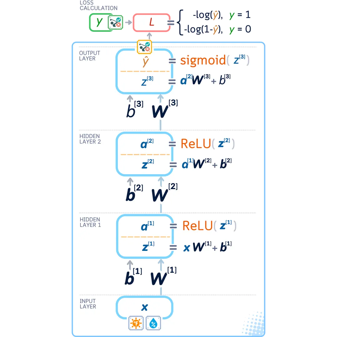
Let’s look at a diagram that shows all the mathematical operations happening in the network. Each layer has:

• Weights ( W ) and Biases ( b ) connecting the layers
• Values before activation ( z )
• Values after activation ( a )
• Final predictions ( ŷ ) and Loss ( L )

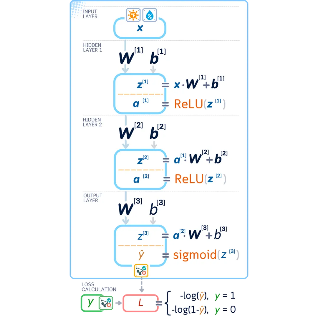
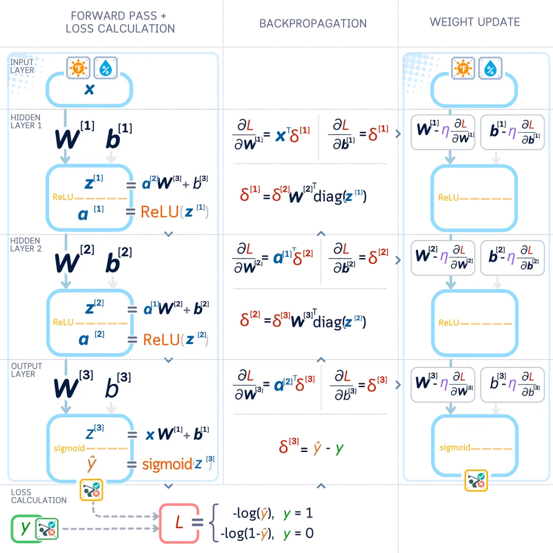
Now let’s see what exactly happens in each layer:

First Hidden Layer:

• Take input x, multiply it by weights W [1], add bias b[1] to get z[1]
• Apply ReLU to z[1] to get output a[1]

Second Hidden Layer:

• Take a[1], multiply it by weights W [2], add bias b[2] to get z[2]
• Apply ReLU to z[2] to get output a[2]

Output Layer:

• Take a[2], multiply it by weights W [3], add bias b[3] to get z[3]
• Apply the sigmoid function to z[3] to get the final prediction ŷ

Now that we have seen all the mathematical knowledge in the network, how do we improve these numbers to get better predictions? That’s where backpropagation comes in – it shows us how to adjust weights and biases to reduce errors.

Step 3: Backpropagation

Before we understand how to improve the network, let’s quickly review some mathematical tools we need:

Gradient

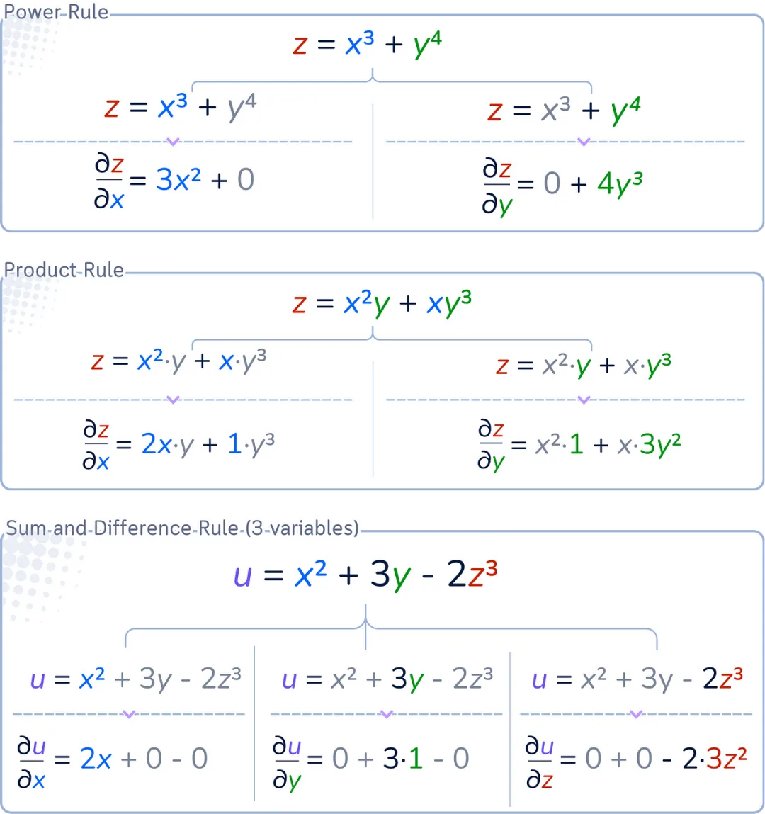
To optimize our neural network, we use gradients – a concept closely related to derivatives. Let’s review some basic derivative rules:

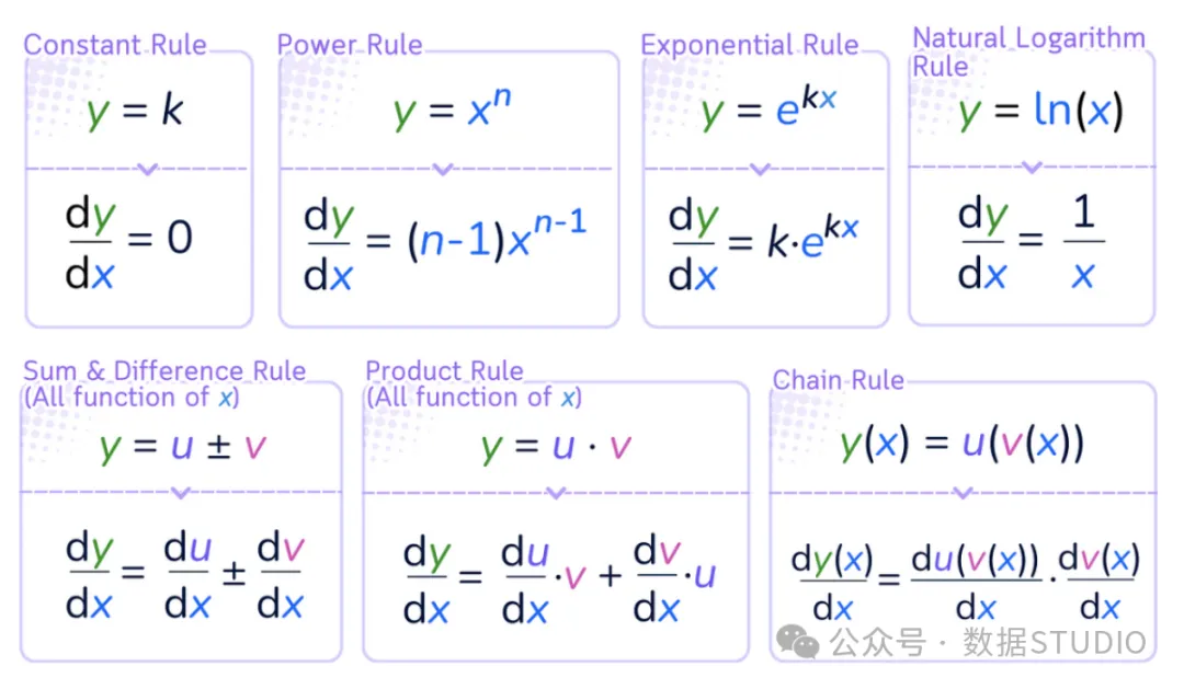
Partial Derivatives

The difference between regular derivatives and partial derivatives:

Regular Derivative:

• Used when the function has only one variable
• Shows the change in the function when its only variable changes
• Written as d f /d x

Partial Derivative:

• Used when the function has multiple variables
• Shows the change in the function when one variable changes while keeping other variables constant.
• Written as ∂f / ∂x

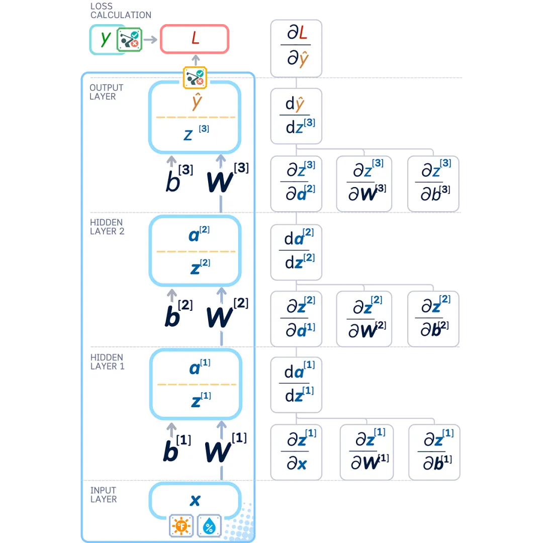
Gradient Calculation and Backpropagation

Going back to our neural network, we need to determine how to adjust each weight and bias to minimize errors. We can use a method called backpropagation to do this, which shows us how changing each value affects our network’s error.

Since backpropagation works backward in our network, let’s flip the diagram upside down to see how it works.

Network Matrix Rules

Since our network uses matrices (groups of weights and biases), we need special rules to compute how changes affect our results. Here are two key matrix rules. For vectors v, u (size 1 × n) and matrices W, X (size n × n):

1. Sum Rule: ∂( W + X )/∂W = I （identity matrix, size n × n） ∂( u + v )/∂v = I （identity matrix, size n × n）
2. Matrix-Vector Product Rule: ∂( vW )/∂ W = v ᵀ ∂( vW )/∂ v = W ᵀ

Using these rules, we get:

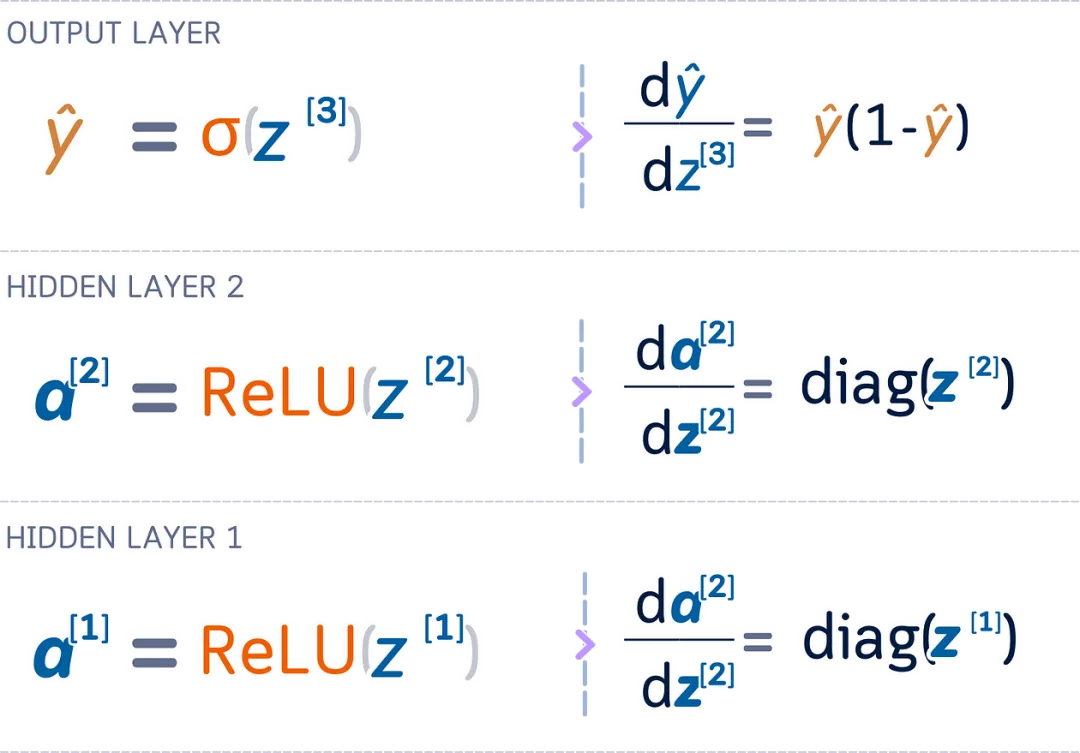
Derivatives of Activation Functions

• Derivative of ReLU

For vector a and z (size 1 × n), where a = ReLU( z ):

∂a /∂z = diag( z > 0)

This creates a diagonal matrix showing: if the input is positive, it is 1; if the input is zero or negative, it is 0.

• Derivative of Sigmoid Function

For a = σ( z ), where σ is the sigmoid function:

∂a / ∂z = a⊙(1 – a )

This directly multiplies the elements (⊙ indicates element-wise multiplication).

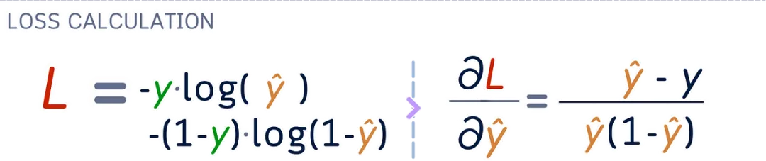
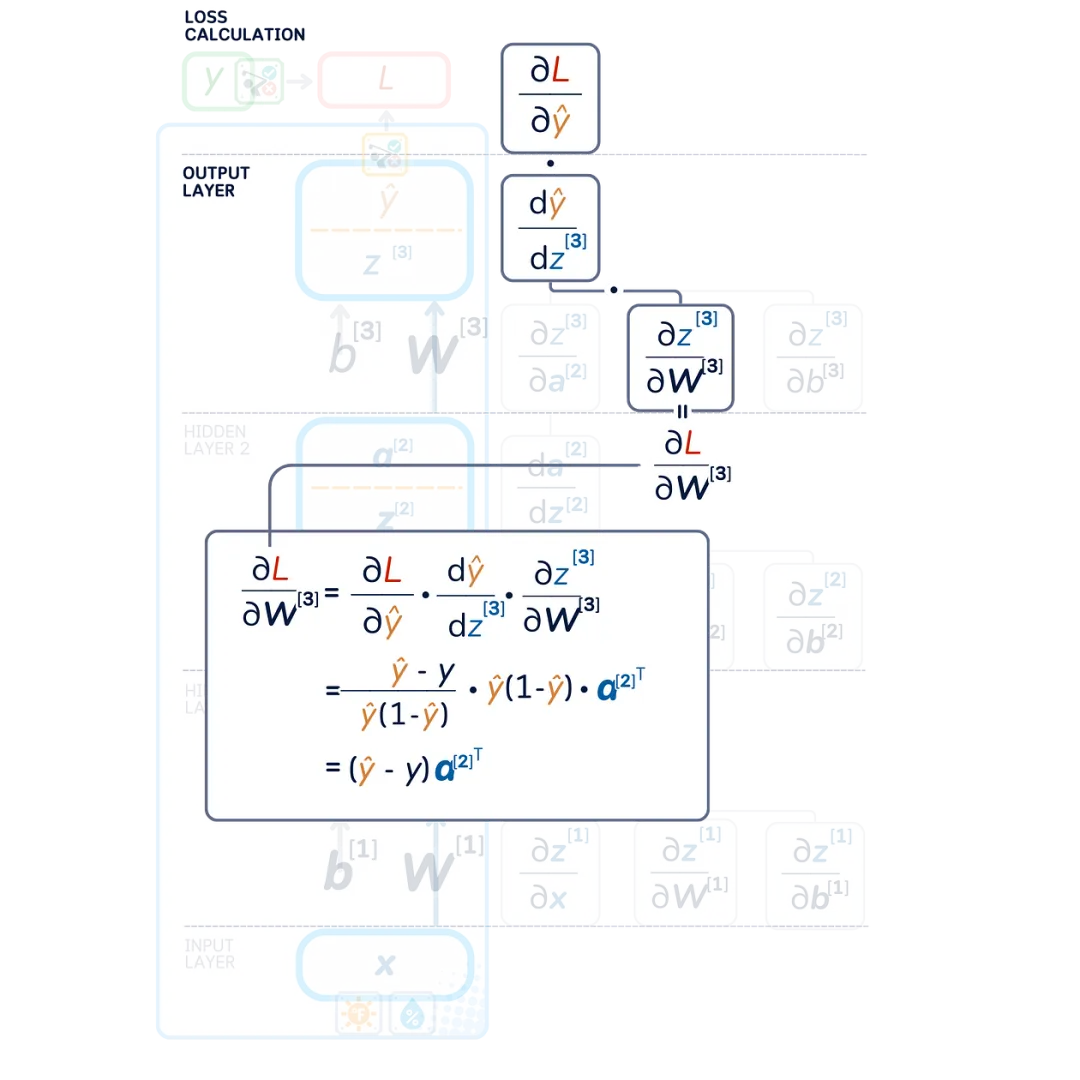
Derivative of Binary Cross-Entropy Loss

For a loss of L = -[ y log(ŷ) + (1- y ) log(1- ŷ )] for a single example:

∂ L /∂ ŷ = -( y – ŷ ) / [ ŷ (1- ŷ )]

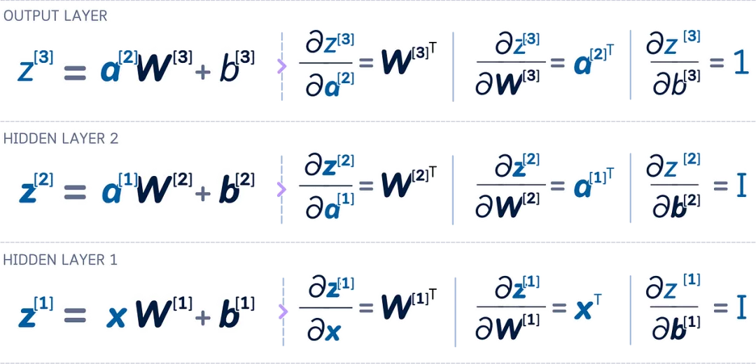
So far, we can summarize all the partial derivatives as follows:

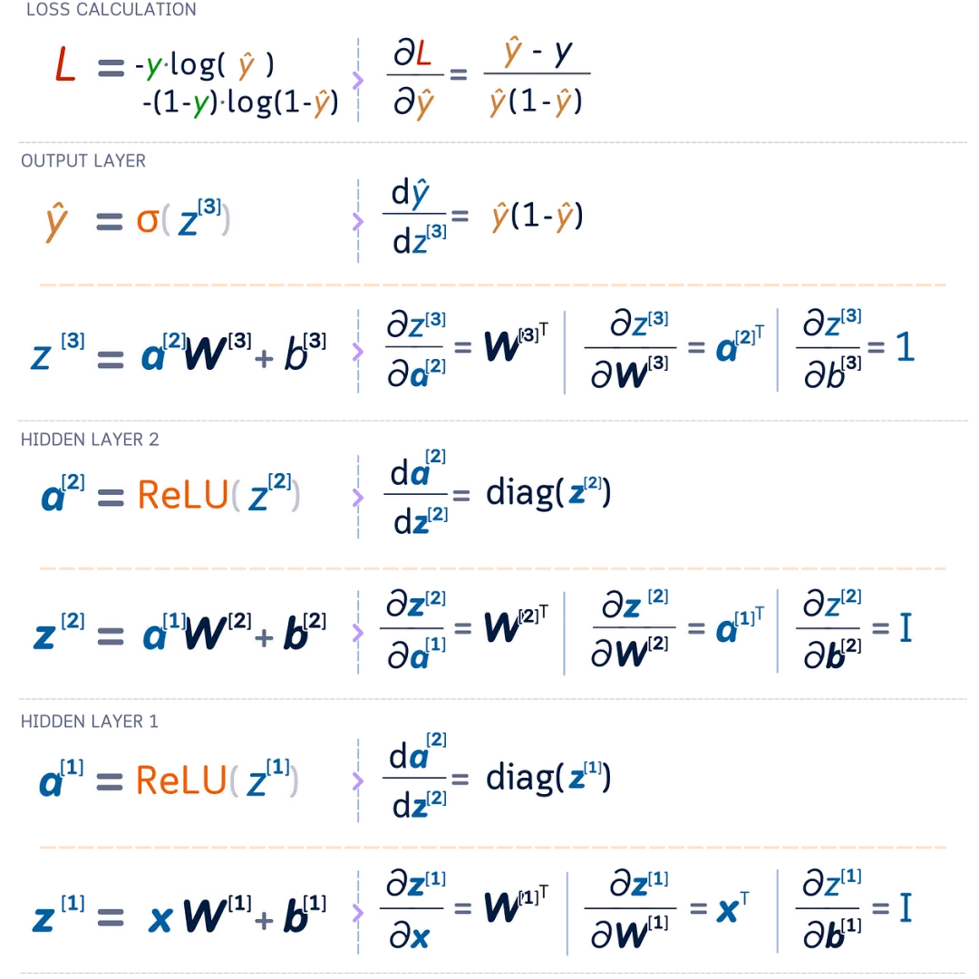
The diagram below shows all the partial derivatives we have obtained so far:

Chain Rule

In our network, the changes propagate through multiple steps: weights affect the output of their layer, which in turn affects the next layer, and so on, until the final error. The chain rule tells us to multiply these stepwise changes to find out how each weight and bias affects the final error.

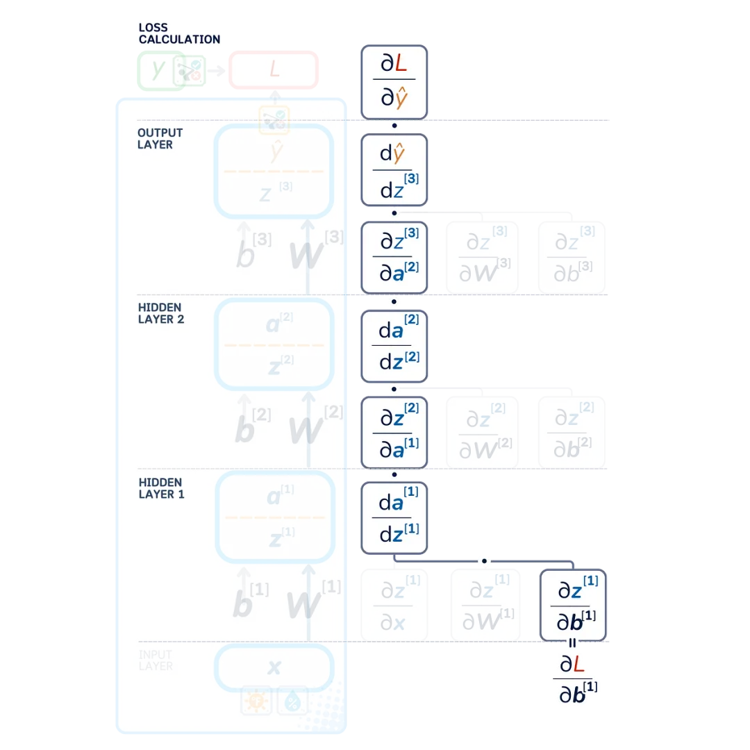
Error Calculation

Instead of directly calculating the derivatives of weights and biases, we first calculate the layer errors ∂ L /∂ zˡ (gradients with respect to the pre-activated outputs). This makes it easier to calculate how to adjust the weights and biases of the previous layers.

Weight Gradients and Bias Gradients

Using these layer errors and the chain rule, we can express the weight and bias gradients as:

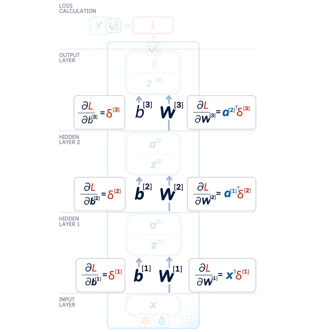
The gradients show us how each value in the network affects the network’s error. We then make slight changes to these values to help our network make better predictions.

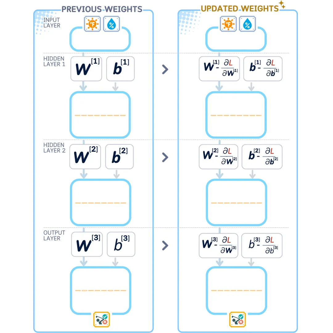
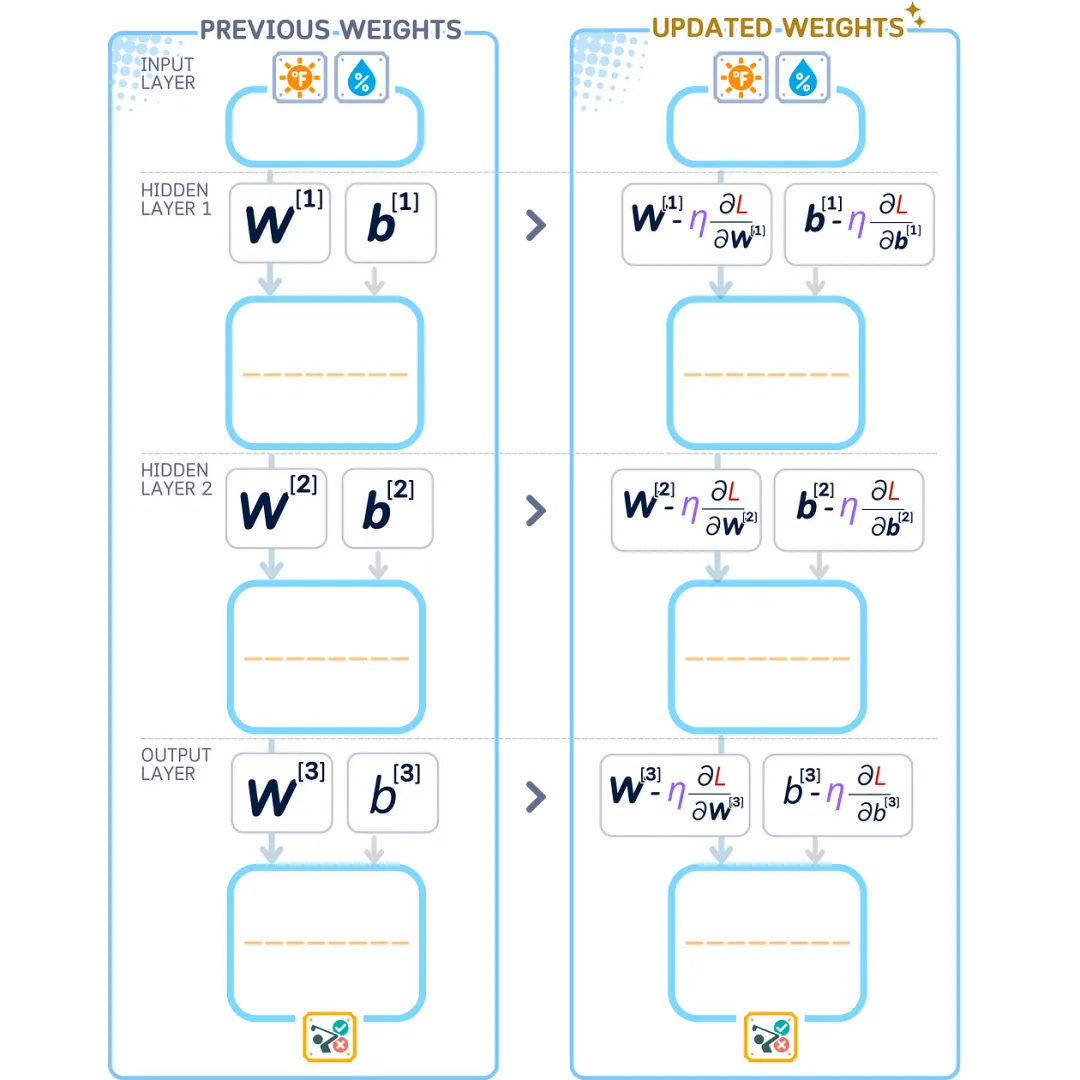
Step 4: Weight Update

Updating Weights

Once we know how each weight and bias affects the error (the gradients), we improve the network by adjusting these values in the opposite direction of the gradient. This gradually reduces the network’s error.

Learning Rate and Optimization

We don’t make large changes all at once, but rather make small, careful adjustments. We use a number called the learning rate ( η ) to control how much each value changes:

• If η is too large: the changes are too big and may make things worse
• If η is too small: the changes are too small and take a long time to improve

This method of making small, controllable changes is called Stochastic Gradient Descent (SGD). We can write it as:

The value of η (learning rate) is typically chosen to be small, usually between 0.1 and 0.0001, to ensure stable learning.

We just saw how our network learns from a single example . The network repeats all these steps for each example in the dataset, getting better with each round of practice.

Step Summary

Here are all the steps we take to train the network based on a single example:

Expanding to Full Dataset

Epoch

Our network repeats these four steps – forward propagation, loss calculation, backpropagation, and weight updates – for each example in the dataset. Going through all examples once is called one epoch.

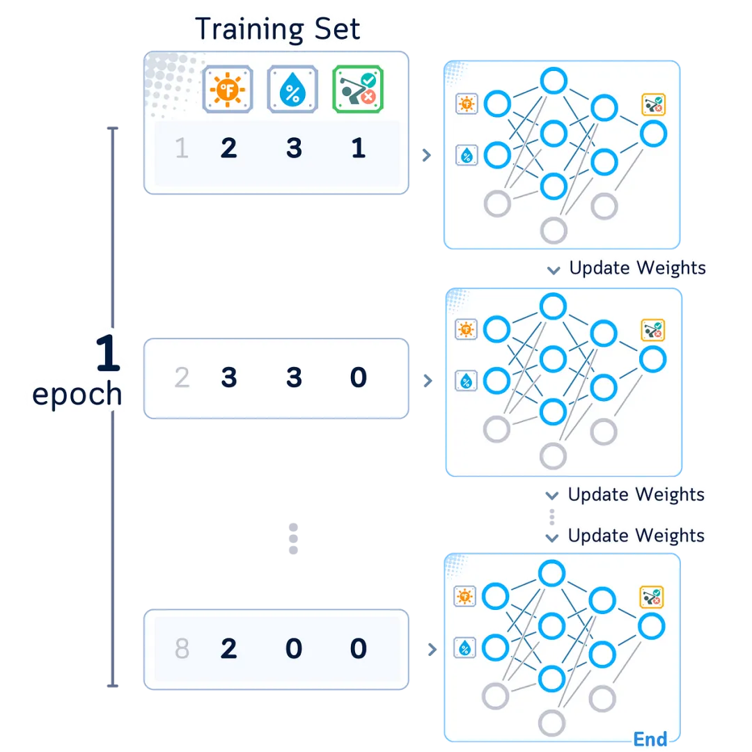
The network often needs to look at all examples multiple times to perform its task well, sometimes even 1000 times. Each pass helps it learn patterns better.

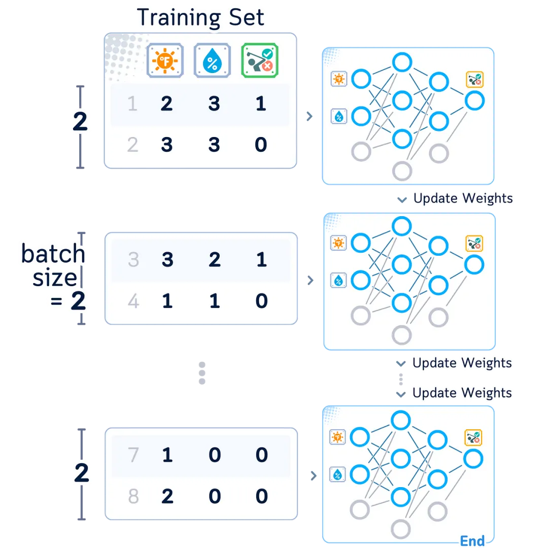
Batch

Our network doesn’t learn from just one example at a time, but rather from a small batch of examples (called batches). This has several benefits:

• Works faster
• Learns better patterns
• Makes more steady progress

When processing batches, the network looks at all examples in the batch before making changes. This leads to better results than changing values after each example.

Testing Steps

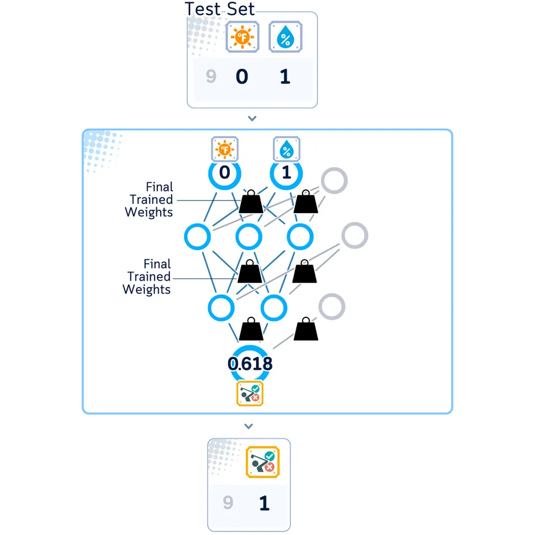
Preparing a Fully Trained Neural Network

After training is complete, our network can make predictions on new examples it has never seen before. It uses the same steps as training but only moves forward through the network to make predictions.

Making Predictions

When processing new data:

1. The input layer accepts new values
2. In each layer:

• Multiply by weights and add biases
• Apply activation function

1. The output layer generates predictions (e.g., probabilities between 0 and 1 for binary classification)

Determinism of Neural Networks

When our network sees the same input twice, it gives the same answer both times (as long as we haven’t changed its weights and biases). The network’s ability to process new examples comes from its training, not from any randomness in the predictions.

Final Thoughts

As our network practices these examples repeatedly, its task gets better and better. Over time, it makes fewer mistakes and its predictions become more accurate. That’s how neural networks learn: by looking at examples, figuring out errors, making small improvements, and then repeating!

Multi-Layer Perceptron Classifier Code Summary

Now let’s see how the neural network works. Below is some Python code that builds the network we’ve been discussing using the same structure and rules we just learned.

import pandas as pd
import numpy as np
from sklearn.neural_network import MLPClassifier
from sklearn.metrics import accuracy_score

# Create a simple 2D dataset
df = pd.DataFrame({ 
    '🌞' : [ 0 , 1 , 1 , 2 , 3 , 3 , 2 , 3 , 0 , 0 , 1 , 2 , 3 ], 
    '💧' : [ 0 , 0 , 1 , 0 , 1 , 2 , 3 , 3 , 1 , 2 , 3 , 2 , 1 ], 
    'y' : [ 1 , - 1 , - 1 , - 1 , 1 , 1 , 1 , - 1 , - 1 , 1 , 1 , 1 ] }, 
    index= range ( 1 , 14 )) 
# Split into training and testing sets
train_df, test_df = df.iloc[:8].copy(), df.iloc[8:].copy()
X_train, y_train = train_df[['🌞', '💧']], train_df['y']
X_test, y_test = test_df[['🌞', '💧']], test_df['y']
# Create and configure our neural network
mlp = MLPClassifier(hidden_layer_sizes=( 3 , 2 ), # Create 2-3-2-1 architecture as described    
       activity= 'relu' ,          # ReLU activation for hidden layers
              resolver= 'sgd' ,               # Stochastic gradient descent optimizer
              learning_rate_init= 0.1 ,     # Step size for weight updates
              max_iter= 1000 ,              # Maximum iterations
              motion= 0 ,                  # Disable pure SGD momentum as described
              random_state= 42             # For reproducible results
) 

# Train the model
mlp.fit(X_train, y_train) 

# Make predictions and evaluate
y_pred = mlp.predict(X_test) 
accuracy = accuracy_score(y_test, y_pred) 
print(f"Accuracy: {accuracy:.2f}")

For reference links, click on the bottom left corner to read the original text. For academic sharing only, if there is any infringement, please delete immediately.