The Rise and Fall of Neural Networks in the 1990s

Excerpt from andreykurenkov

Author: Andrey Kurenkov

Translated by Machine Heart

Contributors: salmoner, Electronic Sheep, Sister Niu Niu, Ben, Slightly Chubby

This is part three of the History of Neural Networks and Deep Learning (see Part One, Part Two). In this section, we will continue to explore the rapid development of research in the 1990s and clarify the reasons why neural networks lost much favor at the end of the 1960s.

1. History of Neural Networks and Deep Learning (Part One): From Perceptrons to BP Algorithm

2. History of Neural Networks and Deep Learning (Part Two): Another Breakthrough After BP Algorithm – Belief Networks

Neural Networks Making Decisions

After the discovery journey of neural networks in unsupervised learning, let’s quickly understand how they are used in the third branch of machine learning: reinforcement learning. A formal explanation of reinforcement learning requires many mathematical symbols, but it has a goal that can be informally described: learning to make good decisions. Given some theoretical agents (like a small software), allow the agent to take actions based on the current state, each action taken will receive some reward, and each action also aims to maximize long-term utility.

Thus, while supervised learning tells the learning algorithm exactly what it should learn to output, reinforcement learning provides rewards over time as a byproduct of good decisions, without directly telling the algorithm what the correct decision should be. From the beginning, this is a very abstract decision model – a finite number of states, and a known set of actions, with known rewards for each state. To find a set of optimal actions, writing a very elegant equation becomes simple, but this is difficult to apply to real problems – those where states persist or rewards are hard to define.

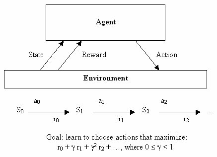Reinforcement Learning

This is where neural networks became popular. Machine learning, in general, especially neural networks, is very good at handling chaotic continuous data or functions that are difficult to define through instance learning. Although classification is the forte of neural networks, they are general enough to solve many types of problems – for example, the Adaline derivatives from Bernard Widrow and Ted Hoff were used for adaptive filters in circuit environments.

Therefore, shortly after the revival of BP research, methods were designed to use neural networks for reinforcement learning. One of the early examples was solving a simple yet classic problem: balancing a stick on a moving platform, a control problem familiar to students in class.

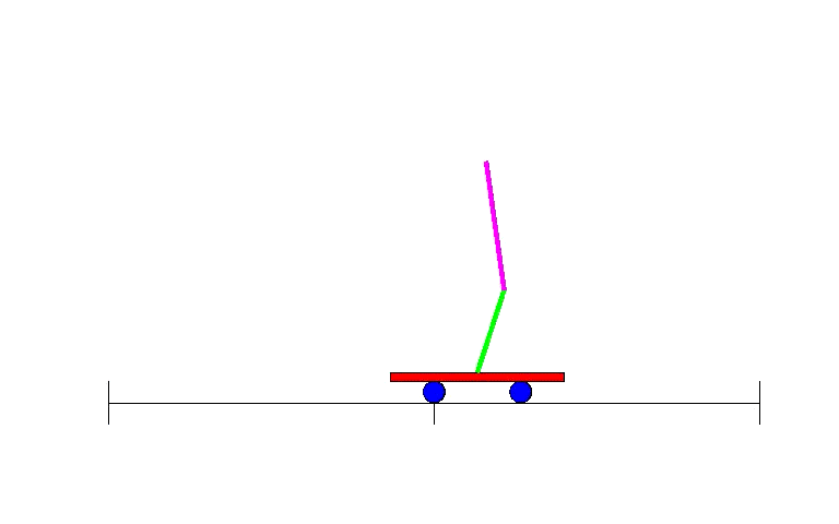The Double Pendulum Control Problem – an advanced version of the single pendulum problem, is a classic control and reinforcement learning task.

Due to adaptive filtering, this research is closely related to the field of electronic engineering, which had become a major subfield in the decades before the emergence of neural networks. Although this field had designed many methods to solve problems through direct analysis, there was also a way to learn to solve more complex states, which proved useful – in 1990, the paper “Identification and control of dynamical systems using neural networks” received 7000 high citations as proof. It can be concluded that there is another independent field from machine learning, where neural networks are useful in robotics. One of the early examples of neural networks used in robotics is the CMU NavLab, the 1989 paper “Alvinn: An autonomous land vehicle in a neural network”:

1. “NavLab 1984 – 1994”

As discussed in the paper, the neural network in this system learned to control the vehicle using sensors and driving data recorded during human driving through ordinary supervised learning. There is also research teaching robots to use reinforcement learning, as demonstrated in the 1993 doctoral thesis “Reinforcement learning for robots using neural networks”. The thesis showed that robots could learn some actions, such as walking along walls or passing through doors within a reasonable timeframe, which was a good thing considering the previously impractically long training times required for the inverted pendulum work.

These applications in other fields are certainly cool, but most research on reinforcement learning and neural networks occurs within artificial intelligence and machine learning. Moreover, we also achieved one of the most significant milestones in the history of reinforcement learning within this scope: a neural network that learned and became a world-class player in backgammon. Researchers trained this neural network, known as TD-Gammon, using standard reinforcement learning algorithms, which also provided the first evidence that reinforcement learning could outperform humans in relatively complex tasks. Furthermore, this is a particularly enhanced learning method, and a similar system that only used neural networks (without reinforcement learning) did not perform as well.

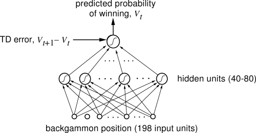A neural network mastering expert-level skills in the game of backgammon

However, as previously seen, we will see again in the field of artificial intelligence that research entered a deadlock. The next problem to be solved using the TD-Gammon method was studied by Sebastian Thrun in 1995 in “Learning To Play the Game of Chess”, with unsatisfactory results. Although the neural network performed well, it was certainly better than a beginner, but it fell short compared to the standard computer program GNU-Chess that had been implemented long ago. Another long-standing challenge for artificial intelligence – Go – was no different. To put it bluntly, TD-Gammon had a bit of an unfair advantage – it learned to evaluate positions accurately, thus requiring no search for many subsequent moves, only selecting moves that could occupy the next most advantageous position. However, in chess and Go games, these games pose a challenge for artificial intelligence because they require estimating many moves, and the possible combinations of actions are so vast. Moreover, even if the algorithms were smarter, the hardware of the time could not keep up, with Thrun stating, “NeuroChess is not great because it spends most of its time evaluating the board. Computing large neural network functions takes twice as long as evaluating optimized linear evaluation functions, like GNU-Chess.” At that time, the inadequacy of computers to meet the demands of neural networks was a very real issue, and as we will see, this was not the only one…

Neural Networks Become Dull

Although unsupervised learning and reinforcement learning are straightforward, supervised learning remains my favorite application of neural networks. Admittedly, learning probability models of data is cool, but solving practical problems through backpropagation is far more exciting. We have seen Yann Lecun successfully solve the problem of recognizing handwritten text (a technique that continues to be used nationwide to scan checks, with even more uses later), while another obvious and quite important task was simultaneously underway: understanding human speech.

Like recognizing handwritten text, understanding human speech is challenging, as the same word can have many different meanings depending on the expression. However, there are additional challenges: long sequences of input. You see, if it’s an image, you can cut out letters from the picture, and then the neural network can tell you what that letter is, in an input-output mode. But language is not that easy; it is completely impractical to break down speech into letters, and even identifying words within speech is not easy. Moreover, think about it, understanding words in context is easier than understanding single words! Although the input-output mode is quite effective for processing images one by one, it does not apply to long information, such as audio or text. Neural networks lack the memory needed to process one input affecting another in sequence, but this is exactly how we humans process audio or text – inputting a string of words or sounds, rather than individual inputs. The point is: to solve the problem of understanding speech, researchers attempted to modify neural networks to handle a series of inputs (as in speech) rather than batch inputs (as in images).

One of the solutions proposed by Alexander Waibel et al. (and Hinton) was introduced in the 1989 paper “Phoneme recognition using time-delay neural networks”. These time-delay neural networks are very similar to conventional neural networks, except that each neuron processes only a subset of inputs, and several sets of weights are equipped for different types of input data delay. In simpler terms, for a series of audio inputs, a “moving window” of audio is input into the neural network, and as the window moves, each neuron with several sets of different weights will assign corresponding weights based on the position of that segment of audio in the window, using this method to process audio. It’s easier to understand with a diagram:

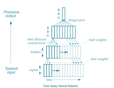Time-Delay Neural Networks

In a sense, this is similar to convolutional neural networks – each unit looks at one subset of inputs at a time, performing the same operation on each small subset, rather than calculating the entire set at once. The difference is that there is no concept of time in convolutional neural networks; the input window of each neuron forms the entire input image to compute a result, while in time-delay neural networks, there is a series of inputs and outputs. An interesting fact: according to Hinton, the idea of time-delay neural networks inspired LeCun to develop convolutional neural networks. However, amusingly, convolutional neural networks became crucial for image processing, while time-delay neural networks lost out to another approach – recurrent neural networks (RNNs). You see, all the neural networks discussed so far are feedforward networks, meaning that the output of a neuron is the input to the next layer of neurons. But it doesn’t have to be this way; there’s nothing stopping us brave computer scientists from connecting the output of the last layer back to the input of the first layer or connecting the output of a neuron back to itself. By looping neurons back into the neural network, memory is elegantly incorporated into the neural network.

Recurrent Neural Network Diagram. Remember the Boltzmann Machine we discussed earlier? Surprised, right? Those are recurrent neural networks.

However, this is not so easy. Consider this problem – if backpropagation relies on “forward propagation” to feed back the errors from the output layer, then how does the system work if the first layer connects back to the output layer? Errors will continue to propagate back to the first layer and then back to the output layer, cycling endlessly in the neural network. The solution is to independently derive multiple groups through time for backpropagation. Basically, this means treating each loop through the neural network as input for another neural network, and limiting the number of loops, thereby unfolding the recurrent neural network.

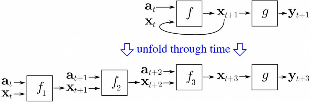An intuitive diagram of backpropagation through time.

This very simple idea really works – training recurrent neural networks is possible. And many people have explored the application of RNNs in language recognition. However, you may have heard of some of the setbacks: this method does not perform very well. To find out why, let’s meet another giant of deep learning: Yoshua Bengio. Around 1986, he began researching neural networks for language recognition and was involved in many academic papers using ANNs and RNNs for language recognition, eventually working at AT&T BELL Labs, where Yann LeCun was also tackling CNNs. In fact, in 1995, the two jointly published the paper “Convolutional Networks for Images, Speech, and Time-Series”, marking their first collaboration, which later led to many joint efforts. However, as early as 1993, Bengio published “A Connectionist Approach to Speech Recognition”. In it, he summarized the general errors of effectively training RNNs:

Although in many examples, recurrent networks can outperform static networks, they are also more difficult to optimize for training. Our experiments tend to show that the parameter adjustments of (recurrent neural networks) often converge to sub-optimal solutions, which only consider short-term effects and do not account for long-term effects. For example, in the described experiments, we found that RNNs fail to capture the simple temporal constraints of single phonemes… Although this is a negative result, better understanding of this issue can help design alternative systems to train neural networks to learn to map input sequences to output sequences with long-term dependencies, such as learning finite state machines, grammars, and other language-related tasks. Since gradient-based methods are clearly insufficient to solve such problems, we need to consider other optimal approaches, arriving at acceptable conclusions even when the criterion function is not smooth.

A New Dawn of Winter

So, there is a problem. A big problem. And fundamentally, this problem is a recent monumental achievement: backpropagation. Convolutional neural networks play a very important role here because backpropagation does not perform well in general neural networks with many layers. However, a key to deep learning is – many layers, with current systems having about 20 layers. However, in the late 1980s, it was found that using backpropagation to train deep neural networks did not yield satisfactory results, especially not as good as training networks with fewer layers. The reason is that backpropagation relies on finding the errors in the output layer and continuously attributing the source of the errors to the previous layers. However, with such a large number of layers, this mathematically based attribution ultimately leads to either a maximum or minimum result, known as the “vanishing or exploding gradient problem”. Jurgen Schmidhuber – another authority in deep learning, provided a more formal and profound summary:

A scholarly paper (published in 1991, authored by Hochreiter) provided a milestone description of deep learning research. Sections five and six of the paper mention that by the late 1990s, some experiments indicated that training feedforward or recurrent deep neural networks with backpropagation was very difficult (see 5.5). Hochreiter pointed out one of the main reasons leading to the problem: traditional deep neural networks encounter the vanishing or exploding gradient problem. Under standard activation conditions (see 1), the accumulated backpropagation error signals either rapidly shrink or exceed limits. In fact, they decay or explode geometrically with the increase of layers or CAP depth (rendering effective training of neural networks nearly impossible).

Flattening the BP path through time is essentially the same as having many layers in a neural network, so training recurrent neural networks with backpropagation is quite challenging. Sepp Hochreiter and Yoshua Bengio, guided by Schmidhuber, have written papers indicating that learning long-term information is not feasible due to the limitations of backpropagation. After analyzing the problem, there are indeed solutions; Schmidhuber and Hochreiter introduced a very important concept in 1997 that ultimately solved the problem of how to train recurrent neural networks: Long Short-Term Memory (LSTM). In short, the breakthroughs in convolutional neural networks and LSTM only brought some minor modifications to the normal neural network models:

The basic principle of LSTM is very simple. Some units are known as Constant Error Carousels (CECs). Each CEC uses an activation function f, which is a constant function, and has a connection to itself with a fixed weight of 1.0. Because the derivative of f is constant at 1.0, the error backpropagated through CECs will not vanish or explode (see section 5.9), but will remain unchanged (unless they “flow out” from the CEC to some other place, typically “flowing to” the adaptive part of the neural network). CECs are connected to many non-linear adaptive units (some units have multiplicative activation functions), thus needing to learn non-linear behaviors. The weights of the units change frequently thanks to the error signal propagating through the CECs over time. Why can LSTM networks learn to explore the significance of events that occurred thousands of discrete time steps ago, while previous recurrent neural networks failed for very short time steps? CECs are the main reason.

But this does not help much in solving the larger perceptual problem, which is that neural networks are relatively crude and do not perform well. Working with them is quite troublesome – computers are not fast enough, and algorithms are not smart enough, leading to dissatisfaction. So around the 1990s, a new AI winter began for neural networks – society lost faith in them again. A new method, known as Support Vector Machines (SVM), was developed and gradually found to outperform the previously tricky neural networks. Simply put, Support Vector Machines mathematically optimize training equivalent to a two-layer neural network. In fact, in 1995, a paper by LeCun, “Comparison of Learning Algorithms For Handwritten Digit Recognition”, already discussed how this new method worked better than the best neural networks at the time, at least performing equally well.

Support Vector Machine classifiers have excellent accuracy, which is their most notable advantage, as they perform well compared to other high-quality classifiers without prior knowledge of the problem. In fact, if a fixed mapping is arranged to the pixels of an image, this classifier will also perform well. Compared to convolutional networks, it is still slow and occupies a lot of memory. But since the technology is still relatively new, improvements are expected.

Other new methods, especially Random Forests, have also proven to be very effective and have strong mathematical theory backing them. Therefore, although recurrent neural networks always perform well, enthusiasm for neural networks gradually waned, and the machine learning community once again denied them. Another winter has arrived. In part four, we will see a small group of researchers who will navigate this bumpy road and ultimately present deep learning to the public in its current form.

References:

1. Anderson, C. W. (1989). Learning to control an inverted pendulum using neural networks. Control Systems Magazine, IEEE, 9(3), 31-37.

2. Narendra, K. S., & Parthasarathy, K. (1990). Identification and control of dynamical systems using neural networks. Neural Networks, IEEE Transactions on, 1(1), 4-27.

3. Lin, L. J. (1993). Reinforcement learning for robots using neural networks (No. CMU-CS-93-103). Carnegie-Mellon Univ Pittsburgh PA School of Computer Science.

4. Tesauro, G. (1995). Temporal difference learning and TD-Gammon. Communications of the ACM, 38(3), 58-68.

5. Thrun, S. (1995). Learning to play the game of chess. Advances in neural information processing systems, 7.

6. Schraudolph, N. N., Dayan, P., & Sejnowski, T. J. (1994). Temporal difference learning of position evaluation in the game of Go. Advances in Neural Information Processing Systems, 817-817.

7. Waibel, A., Hanazawa, T., Hinton, G., Shikano, K., & Lang, K. J. (1989). Phoneme recognition using time-delay neural networks. Acoustics, Speech and Signal Processing, IEEE Transactions on, 37(3), 328-339.

8. Yann LeCun and Yoshua Bengio. 1998. Convolutional networks for images, speech, and time series. In The handbook of brain theory and neural networks, Michael A. Arbib (E()d.). MIT Press, Cambridge, MA, USA 255-258.

9. Yoshua Bengio, A Connectionist Approach To Speech Recognition Int. J. Patt. Recogn. Artif. Intell., 07, 647 (1993).

10. J. Schmidhuber. “Deep Learning in Neural Networks: An Overview”. “Neural Networks”, “61”, “85-117”. http://arxiv.org/abs/1404.7828

11. Hochreiter, S. (1991). Untersuchungen zu dynamischen neuronalen Netzen. Diploma thesis, Institutfur Informatik, Lehrstuhl Prof. Brauer, Technische Universitat Munchen. Advisor: J. Schmidhuber.

12. Bengio, Y.; Simard, P.; Frasconi, P., “Learning long-term dependencies with gradient descent is difficult,” in Neural Networks, IEEE Transactions on , vol.5, no.2, pp.157-166, Mar 1994

13. Sepp Hochreiter and Jürgen Schmidhuber. 1997. Long Short-Term Memory. Neural Comput. 9, 8 (November 1997), 1735-1780. DOI=http://dx.doi.org/10.1162/neco.1997.9.8.1735.

14. Y. LeCun, L. D. Jackel, L. Bottou, A. Brunot, C. Cortes, J. S. Denker, H. Drucker, I. Guyon, U. A. Muller, E. Sackinger, P. Simard and V. Vapnik: Comparison of learning algorithms for handwritten digit recognition, in Fogelman, F. and Gallinari, P. (Eds), International Conference on Artificial Neural Networks, 53-60, EC2 & Cie, Paris, 1995

© This article is originally compiled by Machine Heart, please contact this account for authorization to reproduce.

✄————————————————

Join Machine Heart (Full-time Reporter/Intern): [email protected]

Submissions or inquiries: [email protected]

Advertising & Business Cooperation: [email protected]

Machine Heart is a Comet Labs cutting-edge technology media. Comet Labs is a global AI and smart machines acceleration investment platform initiated and independently operated by Lenovo Star, collaborating with leading industry companies and investment institutions worldwide to help entrepreneurs solve key issues such as industry docking, user expansion, global market, technology integration, and funding. Its businesses also include: Comet San Francisco Accelerator, Comet Beijing Accelerator, Comet Vertical Industry Accelerator.

↓↓↓ Click “Read the Original” to view the Machine Heart website for more exciting content.