1 Introduction
Deep neural networks are composed of neurons organized into layers and interconnected, capturing their architecture through computation graphs, where neurons are represented as nodes and directed edges connect different layers of neurons. The performance of neural networks depends on their architecture, but there is currently a lack of systematic understanding of the relationship between the accuracy of neural networks and the underlying graph structure. This directly affects the design of more efficient and precise architectures and can inform new hardware architecture designs. Establishing the relationship between neural network architecture and its accuracy is of significant scientific and practical importance, but it remains unclear how to map neural networks to graphs. Computation graph representations have many limitations, such as lack of generality and disconnection from biology/neuroscience.
Stanford’s Jure Leskovec and Facebook’s He Kaiming and others have developed a new method to represent neural networks as graphs, called relational graphs, focusing on message exchange rather than just data flow. This representation can represent many types of neural network layers while freeing itself from many constraints of computation graphs.
This work designed a graph generator called WS-flex, capable of systematically exploring the design space of neural networks, as shown in Figure 1. Using standard image classification datasets CIFAR-10 and ImageNet, a systematic study was conducted on how neural network architecture affects its predictive performance, leading to several important empirical observations:
(1) Specific points in the relational graph can significantly enhance the predictive performance of neural networks;
(2) The performance of neural networks is closely related to the clustering coefficient and average path length of their relational graphs, presenting a smooth functional relationship;
(3) The findings of this paper are applicable to various tasks and datasets, demonstrating broad applicability;
(4) The ability to effectively identify optimal points;
(5) The best-performing neural networks exhibit a high degree of similarity in graph structure to real biological neural networks.
These results have important implications for designing neural network structures, advancing deep learning science, and enhancing understanding of neural networks.
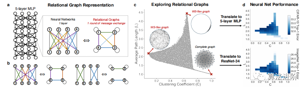
Figure 1 Overview of our method. (a) A layer of a neural network can be viewed as a relational graph, where we connect nodes that exchange messages. (b) More examples of neural network layers and relational graphs. (c) We explore the design space of relational graphs based on graph metrics (including average path length and clustering coefficient), where the complete graph corresponds to a fully connected layer. (d) We transform these relational graphs into neural networks and study how their predictive performance depends on the corresponding graph metrics.
2 Neural Networks as Relational Graphs
This section introduces the concept of relational graph representation and its instantiation, demonstrating how to capture different neural network architectures using a unified framework. Using graph language in the context of deep learning helps bridge the two worlds and lays the foundation for research.
2.1 Message Exchange Through Graphs
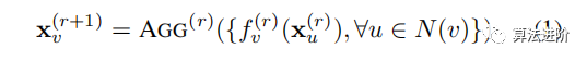
This paper defines a neural network graph G=(V,E), where V is the set of nodes and E is the set of edges. Suppose node v has a feature vector xv. When graph G is related to neuron message exchange, it is called a relational graph. Message exchange is defined by a message function and an aggregation function, where in each round of message exchange, each node sends messages to its neighbors and aggregates incoming messages from neighbors. Each message is transformed through the message function f(·) along each edge and then aggregated at each node through the aggregation function AGG(·). Assuming R rounds of message exchange are conducted, the r-th round message exchange for node v can be described as
where u, v are nodes in graph G, N(v) is the neighborhood of node v, including self-loops. x(v) is the input node features, and x(v+1) is the output node features. This method can be defined on any graph G, and this paper only considers undirected graphs.
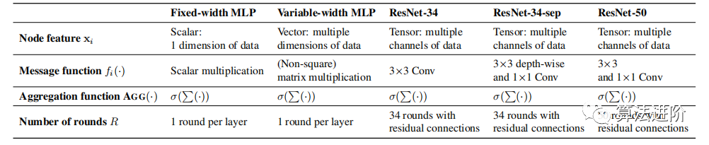
Equation 1 defines message exchange, and subsequent discussions focus on how to apply it to different neural architectures. Table 1 summarizes various instantiations, and Figure 2 illustrates a specific example of a 4-layer 65-dimensional MLP.
Table 1 Various neural architectures expressed in relational graph language. These architectures are typically realized as complete relational graphs, and we systematically explore more graph structures of these architectures.
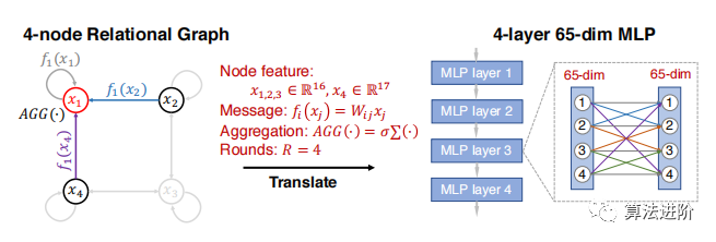
Figure 2 Example of converting a 4-node relational graph into a 4-layer 65-dimensional MLP. We highlight the message exchange of node x1. Using different definitions of xi, fi(·), AGG(·), and R (as defined in Table 1), relational graphs can be transformed into different neural architectures.
2.2 Fixed-Width MLPs as Relational Graphs
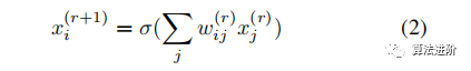
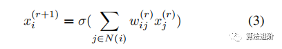
Multi-layer perceptrons (MLPs) consist of layers of computational units (neurons), where each neuron performs a weighted sum on scalar inputs and outputs, followed by non-linear processing. Suppose the r-th layer of the MLP takes x(r) as input and produces x(r+1) as output. The neuron computes:
where w(r)ij are trainable weights, x(r)j is the j-th dimension of input x(r), x(r+1)i is the i-th dimension of output x(r+1), and σ is the non-linearity.
Under special conditions, all layers x(r) have the same feature dimension for input and output. In this case, fully connected, fixed-width MLP layers can be represented as relational graphs, where each node xi connects to all other nodes. Fully connected fixed-width MLP layers have a special definition of message exchange, where the message function is fi(xj)=wijxi, and the aggregation function is AGG({xi})=σ(P{xi}).
The above discussion indicates that fixed-width MLPs can be viewed as complete relational graphs with special message exchange capabilities, a special case under a more general family of models where the message function, aggregation function, and relational graph structure can vary.
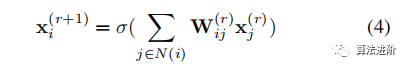
This insight generalizes fixed-width MLPs to any general relational graph G, based on the general definition of message exchange in Equation 1:
where i, j are nodes in G, and N(i) is defined by G.
2.3 General Neural Networks as Relational Graphs
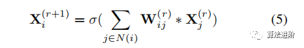
This section discusses how to extend relational graphs to general neural networks, particularly variable-width MLPs. In CNNs, layer widths (number of feature channels) vary, thus necessitating the extension of node features from scalar x(r)i to vector x(r)i, composed of certain dimensions of the MLP input x(r), and the message function fi(·) from scalar multiplication to matrix multiplication:
where W(r)ij is the weight matrix, allowing different dimensions for the same node across different layers and different nodes within the same layer, leading to flexible graphical representations of neural networks. For example, using a 4-node relational graph to represent a 2-layer neural network, the first layer width is 5, and the second layer width is 9, so the sizes of the 4 nodes in the first layer are {2,1,1,1}, and in the second layer are {3,2,2,2}.
The maximum number of nodes in the relational graph is limited by the narrowest layer width in the neural network, with each node’s feature dimension being at least 1.
Relational Graphs as CNNs.Node features are extended from vector x(r)i to tensors X(r)i composed of some channels from the input image. The message exchange definition is then summarized using convolution operators, specifically:
where ∗ is the convolution operator, and W(r)ij is the convolution filter. In this definition, widely used dense convolutions are again represented as complete graphs.
Modern Neural Architectures as Relational Graphs.We use relational graphs to depict modern neural architectures with complex designs, such as ResNet and neural networks with bottleneck transformations. The residual connections of ResNet are preserved, while bottleneck transformation neural networks alternately apply 3×3 and 1×1 convolution message exchanges. In computationally efficient settings, separable convolutions (alternating 3×3 depth convolutions and 1×1 convolutions) are widely used.
Relational graphs are a universal representation of neural networks, capable of representing various neural architectures through the definition of node features and message exchanges, as shown in Table 1.
3 Exploring Relational Graphs
This section explores how to design and investigate the relationship between neural network graph structures and predictive performance through three key components: (1) graph metrics to characterize graph structural properties; (2) graph generators to produce diverse graphs; (3) methods to control computational budgets to attribute differences in neural network performance.
3.1 Selection of Graph Metrics
Given the complexity of graph structures, graph metrics are often used to characterize graphs. This paper primarily introduces two metrics: global average path length and local clustering coefficient. These two metrics are widely used in neuroscience and network science. The average path length measures the average shortest path distance between any pair of nodes; the clustering coefficient measures the proportion of edges among the neighbors of a given node, averaged over all nodes. Additional graph metrics are available for analysis in the appendix.
3.2 Design of Graph Generators
Our goal is to use graph generators to produce diverse graphs that cover a wide range of graph metrics. However, this requires careful design of the generators, as classical graph generators can only produce limited categories of graphs, while learning-based graph generators aim to mimic given example graphs.
Limitations of Existing Graph Generators.We investigated classical graph generators such as ER, WS, BA, Harary, circular graphs, and complete graphs, finding that the graphs they produce have limited spans in the average path length and clustering coefficient space, indicating limitations in existing graph generators, as shown in Figure 3.
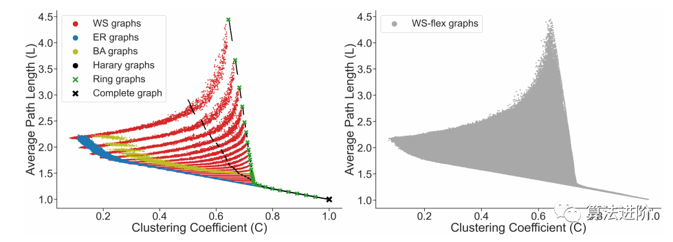
Figure 3 Graphs generated by different graph generators. The proposed graph generator WS-flex can cover a larger area of graph design space. WS (Watts-Strogatz), BA (Barabási-Albert), ER (Erdős-Rényi).
WS-flex Graph Generator.The WS-flex graph generator can generate graphs that cover a wide range of graph metrics, nearly encompassing all graphs generated by classical random generators, as shown in Figure 3. WS-flex achieves this by relaxing the constraint that nodes have the same degree in the WS model. WS-flex is parameterized by the number of nodes n, average degree k, and rewiring probability p, with the number of edges given by e=bn*k/2c. The generator first creates a circular graph, then randomly selects nodes and connects them to their nearest neighbors, and finally randomly rewires edges with probability p. WS-flex samples smoothly in the clustering coefficient and average path length space, experimenting with 3942 graphs, as shown in Figure 1(c).
3.3 Controlling Computational Budgets
To compare the performance differences of different graph-transformed neural networks, we ensure that all networks have approximately the same complexity, using FLOPS as the metric. First, we calculate the FLOPS of the baseline network instantiation as a reference complexity, then adjust the width of the neural networks to match the reference complexity without changing the relational graph structure.
4 Experimental Setup
We studied the graph structures of MLPs on the CIFAR-10 and ImageNet datasets, with CIFAR-10 containing 50K training images and 10K validation images, and ImageNet consisting of 1K image classes, 1.28 million training images, and 50K validation images.
For the CIFAR-10 experiment, we used a 5-layer MLP with 512 hidden units, where the input is a 3072-dimensional flattened vector of (32×32×3) images, and the output is a 10-dimensional prediction. Each layer is equipped with a ReLU non-linear layer and a BatchNorm layer. We adopted a cosine learning rate schedule, starting with a learning rate of 0.1, decaying to 0, without restarts, with a batch size of 128, and trained for 200 epochs. We trained all MLP models using 5 different random seeds and reported average results.
In the ImageNet experiment, we used three architectures from the ResNet series, including ResNet-34, ResNet-34-sep, and ResNet-50, as well as EfficientNet-B0 and an 8-layer CNN. All models were trained for 100 epochs using a cosine learning rate schedule, starting with a learning rate of 0.1. Training the MLP models took 5 minutes on an NVIDIA Tesla V100 GPU, while training the ResNet models on ImageNet took a day.
4.2 Exploration Using Relational Graphs
We instantiated sampled relational graph instances into neural networks using the definitions in Table 1, replacing all dense layers. The input and output layers were kept unchanged, while other designs were retained. We then matched the reference computational complexity of all models, as described in Section 3.3.
In the CIFAR-10 MLP experiment, we explored 3942 sampled relational graphs with 64 nodes, as described in Section 3.2. In the ImageNet experiment, due to higher computational costs, we uniformly subsampled 52 graphs from the 3942 graphs. For EfficientNet-B0, we resampled 48 relational graphs with 16 nodes.
5 Results
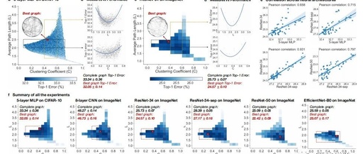
This section summarizes the experimental results, including top-1 errors of sampled relational graphs across different tasks and architectures, along with the graph metrics (average path length L and clustering coefficient C) for each sampled graph. The results are presented in the form of heatmaps relating graph metrics to predictive performance (Figures 4(a)(c)(f)).
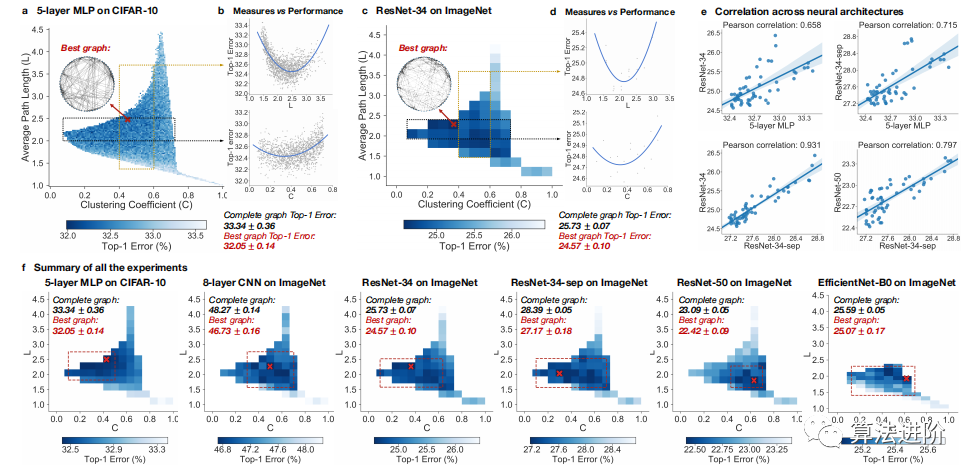
Figure 4 Key Results. The computational budgets for all experiments were strictly controlled. Each visualization result is the average of at least 3 random seeds. The complete graph with C=1 and L=1 (bottom right corner) is treated as the baseline. (a)(c) Graph metrics versus neural network performance. The best graphs significantly outperform the baseline complete graph. (b)(d) Single graph metrics versus neural network performance. Relational graphs falling within a given range are displayed as gray points. The overall smooth function is represented by the blue regression line. (e) Consistency across architectures. The performance correlation of the same set of 52 relational graphs when transformed into different neural architectures is shown. (f) Summary of all experiments. In different settings, the optimal relational graphs (red crosses) consistently outperform the baseline complete graph. Additionally, we highlight the “optimal points” (red rectangular area), where relational graphs are statistically not worse than the best relational graphs (areas with red crosses). The bin values for the 5-layer MLP on CIFAR-10 are the averages of all relational graphs falling within the given bins for C and L.
5.1 Optimal Choices for Top Neural Networks
The heatmap (Figure 4(f)) shows that certain graph structures can surpass the complete graph baseline, enhancing performance. The optimal relational graphs achieve top-1 errors that are 1.4% and 0.5%-1.2% lower than the complete graph baseline on CIFAR-10 and ImageNet, respectively. The best graphs cluster in the optimal locations defined by C and L (the red rectangle in Figure 4(f)). The optimal points were determined through downsampling, aggregation, identifying the bin with the best average performance, one-tailed t-tests, and recording bins that were not significantly different. For the 5-layer MLP on CIFAR-10, the optimal point is Cε[0.10,0.50], Lε[1.82,2.75].
5.2 Neural Network Performance as a Smooth Function of Graph Metrics
Figure 4(f) shows that the predictive performance of neural networks presents a smooth functional relationship with the clustering coefficient and average path length of relational graphs. In Figures 4(b)(d), fixing one graph metric value visualizes network performance based on other metrics. Overall trends are visualized using quadratic polynomial regression, revealing a smooth U-shaped correlation between clustering coefficient, average path length, and neural network performance.
5.3 Consistency Across Architectures
Relational graphs define a shared design space across neural architectures, where relational graphs with certain graph metrics may consistently perform well regardless of their instantiation.
Quality Consistency.Figure 4(f) reveals that the best points across different architectures are roughly consistent, with a cross-architecture optimal point of C∈[0.43,0.50], L∈[1.82,2.28], consistent U-shaped trends between measured values and neural network performance in Figures 4(b)(d).
Quantitative Consistency.To further quantify consistency across tasks and architectures, we selected 52 bins in the heatmap of Figure 4(f), where bin values represent the average performance of relational graphs falling within that bin range for their graph metrics. It was observed that the performance of relational graphs with certain graph metrics correlates across different tasks and architectures.
5.4 Rapid Identification of Optimal Locations
We propose a method to identify optimal points at a lower computational cost by reducing the number of sampled graphs and training epochs.
How Many Graphs Are Needed?
The heatmap (Figure 4(f)) analysis for the 5-layer MLP on CIFAR-10 shows that the bin values calculated from 52 graphs sampled from the 3942 graph samples have a high Pearson correlation of up to 0.90 with the bin values calculated using all 3942 graph samples, as shown in Figure 5 (left). This indicates that far fewer graphs are needed for similar analyses.
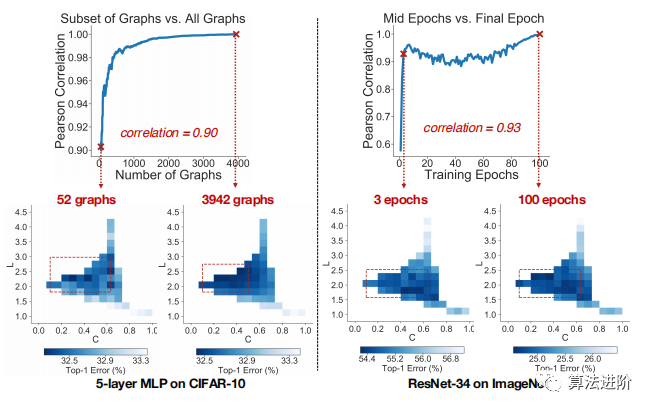
How Many Training Epochs Are Needed?Using ResNet-34 on ImageNet as an example, we calculated the correlation between the validation top-1 error of partially trained models and the validation top-1 error of models trained for 100 epochs, as shown in Figure 5 (right). The results reveal that models trained after just 3 epochs already have a high correlation (0.93). This finding indicates that good relational graphs perform well even in early training epochs, significantly reducing the computational cost of determining whether a relational graph is promising.
5.5 Connections Between Network Science and Neuroscience
Network Science.The average path length we measured reflects the extent of information exchange in the network, consistent with our definition of relational graphs. The U-shaped correlation in Figures 4(b)(d) may indicate a trade-off between message exchange efficiency and the ability to learn distributed representations.
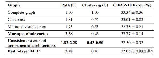
Neuroscience.Our findings reveal that the top-performing relational graphs exhibit a striking similarity to biological neural networks, as shown in Table 2 and Figure 6. The graph metrics of top artificial neural networks are highly similar to those of biological neural networks, and relational graph representations can transform biological neural networks into 5-layer MLPs, outperforming the baseline complete graph. Our approach opens new possibilities for interdisciplinary research across network science, neuroscience, and deep learning.
Table 2 Top artificial neural networks can be similar to biological neural networks
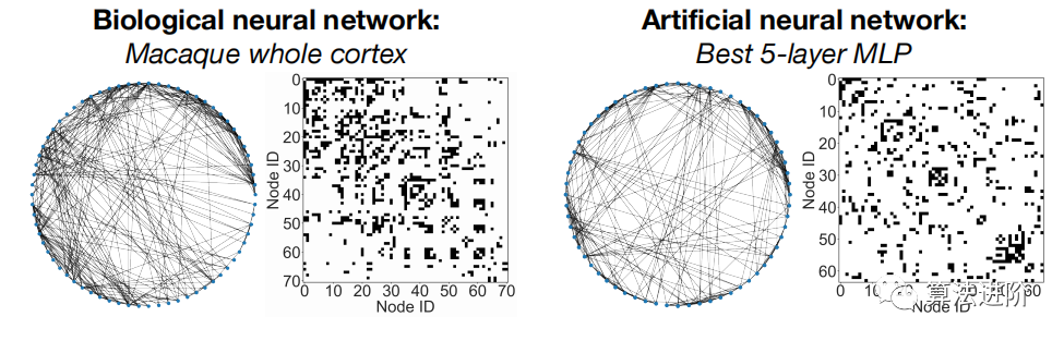
Figure 6 Visualization of biological (left) and artificial (right) neural network graph structures.
6 Related Work
Neural Network Connectivity.The design of neural network connectivity patterns primarily focuses on macro and micro structures. Macro structures concern inter-layer connections, while micro structures focus on intra-layer connectivity. Deep Expander Networks and RandWire utilize expanded graphs and graph generators to create structures but do not explore the statistical relationship between graph structures and network performance. Cross-channel communication networks encourage neurons to communicate through messaging, only considering complete graph structures.
Neural Architecture Search.Research improves learning/search algorithms at either micro or macro levels to learn connectivity patterns. NAS-Bench-101 defines a search space for graphs by enumerating DAGs of constrained size. New pathways define a smooth space using graph generators and graph metrics, reducing search costs without exhaustively searching all possible connectivity patterns.
7 Discussion
Hierarchical Graph Structures of Neural Networks.Our work focuses on hierarchical graph structures at the layer level, which are foundational to neural networks. While exploring this area is computationally challenging, we hope our methods and findings can be generalized.
Efficient Implementation.We utilized standard CUDA kernels, resulting in performance lower than the baseline complete graph. However, we are exploring block-sparse kernels and fast sparse ConvNets to narrow the gap between theoretical FLOPS and actual gains, providing insights for new hardware architecture designs.
Priors and Learning.We use relational graph representations as structural priors, hardwired into the neural network. Deep ReLU neural networks can automatically learn sparse representations. The question remains whether fully connected neural networks exhibit any graph structure without graph priors.
We conducted “reverse engineering” on trained neural networks to study their relational graph structures. Training a fully connected 5-layer MLP on CIFAR-10, we inferred the underlying relational graph structure of the network through specific steps. The results (Figure 7) revealed that the extracted graph after training convergence was no longer an E-R random graph but moved towards the optimal point region. The learned graphs still exhibited a gap from the best graphs imposed as structure, which may explain the poorer performance of fully connected MLPs.
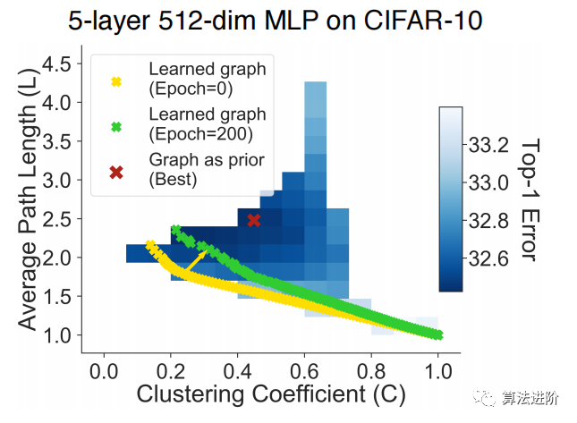
Figure 7 Priors and Learning. Results of a 5-layer MLP on CIFAR-10. We highlight the graph that performs best when used as a structural prior. Additionally, we trained a fully connected MLP and visualized the learned weights as a relational graph (different points represent graphs at different thresholds). The learned graph structure after training moved towards the “optimal point,” but did not close the gap.
Our experimental findings indicate that when tasks are simple and network capacity is rich, learning graph structures can be superior. This suggests that studying the graph structure of neural networks is crucial for understanding their predictive performance.We propose a unified view of Graph Neural Networks (GNN) and general neural architectures, defining neural networks as message exchange functions on graphs. We point out that GNNs are a special form of general neural architectures where graph structures are viewed as inputs rather than as part of the neural architecture.Our work provides a foundation for a unified view of GNNs and general neural architecture design, promising to inspire new innovations.
Follow 👇 the public account and reply 【GS4NN】 to download the related paper
For more exciting content, please click: Selected Articles in AI Field!