Deep Learning Tips for Effective Neural Network Training

Produced by Big Data Digest

Compiled by: Shijin Tian, Ni Ni, Hu Jia, Yun Zhou

In many machine learning labs, machines have undergone thousands of hours of training. During this process, researchers often take many detours and fix many bugs, but it is certain that the experience and knowledge gained during the research process are not only for the machines; we humans also accumulate rich experience. This article will provide you with some of the most practical research suggestions.

This article will introduce some experiences when training deep neural networks (mainly based on the TensorFlow platform). Some suggestions may seem obvious to you, but they may be very important to others. Some suggestions may not apply to certain specific tasks, so please use them with caution!

General Suggestions

Use the ADAM optimizer. Compared to traditional optimizers like batch gradient descent, the Adam optimizer performs better.

TensorFlow usage suggestion: When saving and restoring weights, remember to create the Saver after creating the Adam optimizer, as Adam also has state (also called unit weights of learning rate) that needs to be restored.

ReLU is the best nonlinear mapping (activation function). Just as Sublime is the best text editor, ReLU is fast and simple, and the magic is that it does not gradually reduce the gradient during training. Although sigmoid is commonly used as an activation function in textbooks, it does not transmit gradients well in DNNs.

Do not use an activation function in the output layer. This should be obvious, but if you have used a shared function in every layer of the network, this mistake is common. Make sure you do not use an activation function in the output layer.

Add a bias value in each layer. This is a basic knowledge of machine learning: the essence of bias is to shift a plane to the best fit position. In the function y=mx+b, b is a bias value that can move the line to the best fit position.

Use variance-scaled initialization. In TensorFlow, use methods like tf.contrib.layers.variance_scaling_initializer() for initialization.

In our experience, this method performs better than conventional Gaussian distribution initialization, truncated normal distribution initialization, and Xavier initialization methods.

Overall, variance-scaled initialization can adjust the variance of the initial random weights based on the number of inputs and outputs of each layer (defaulting to the number of inputs in TensorFlow), helping signals to propagate deeper in the network without needing additional methods like truncation or batch normalization.

Xavier initialization is similar but essentially the same across all layers; if the range of values between layers is very different (common in convolutional networks), using the same variance for each layer may not be applicable.

Normalize input data. During training, subtract the mean of the dataset and then divide by the standard deviation. This can reduce the stretching of weights in every direction, helping the neural network learn faster and better. Keeping the input data centered around the mean variance can achieve this well. You should also ensure that the same normalization method is applied to test inputs to ensure that your training set can simulate a real data environment.

Scale data reasonably. This is related to normalization but should be done before normalization. For example, if the data x in real life ranges from [0, 140000000], it may follow a tanh(x) or tanh(x/C) distribution, where C is a constant used to adjust the curve to help input data fit better into the slope part of the tanh function. Especially when your input data is unbounded at one or both ends, the neural network can learn better in the range (0, 1).

Generally, do not bother to reduce the learning rate. Learning rate decay is more common in SGD, but ADAM can handle it more naturally. If you must care about minor performance differences: briefly reduce the learning rate at the end of training, and you may see a sudden drop in error, followed by stabilization.

If your convolutional layer has 64 or 128 filters, this may be excessive, especially for deep networks; 128 filters may be too many. If you already have a large number of filters, adding more may be meaningless.

Pooling is to maximize the invariance of transformations. Pooling essentially allows the neural network to learn the overall features of a part of the image. For example, max pooling can maintain the invariance of features even after transformations like displacement, rotation, and scaling in convolutional networks.

Debugging Neural Networks

If your neural network cannot learn, meaning that the loss or accuracy does not converge during training, or you cannot achieve the expected results, try the following suggestions:

Overfitting! If your network does not converge, the first thing to do is to overfit a training point, aiming for an accuracy of 100% or 99.99%, or an error close to 0. If your neural network cannot overfit a single data point, then there is a serious but possibly subtle problem with your architecture. If you can overfit a data point but cannot converge when training on a larger dataset, then consider the following suggestions.

Lower the learning rate. Your network will learn more slowly, but it can descend to the minimum that it previously could not reach due to the step size being too large. (Imagine finding the minimum being like trying to reach the lowest point in a ditch, but a step size too large causes you to jump over the ditch.)

Increase the learning rate. A larger learning rate helps shorten training time and reduce feedback loops, meaning you can quickly predict whether the network model is feasible. However, while the network model can converge faster, the results may not be particularly ideal and may even have significant oscillations. (We found that for the ADAM optimizer, a learning rate of 0.001 works well in many experiments.)
Reduce the batch size. Using a batch size of 1 can obtain finer granularity of weights for feedback updates; you can use TensorBoard to visualize (or other debugging/visualization tools).
Remove batch normalization. As the batch size is reduced to 1, removing batch normalization can expose issues of vanishing or exploding gradients. We had a neural network model that still could not converge after several weeks. It wasn’t until we removed batch normalization that we realized all outputs became NaN after the second iteration. Batch normalization acts like a band-aid for bleeding, but it only works if your network model has no errors.
Increase the batch size. A larger batch size, such as using the entire dataset, reduces the variance of gradient updates, making the results of each iteration more precise. In other words, weight iterations will move in the right direction. However, this method is limited by physical memory size. Generally, the first two techniques using a batch size of 1 and removing batch normalization are more useful than this technique.
Check matrix reshaping. Large matrix reshaping (e.g., changing the aspect ratio of images) can disrupt the locality of spatial features, making it harder for the model to learn because reshaping is also a part that needs to be learned. (Natural features become fragmented. In fact, the spatial locality of natural features is also why convolutional neural networks are effective.) Pay special attention to multi-graph/channel matrix reshaping; use numpy.stack() for appropriate adjustments.
Check the loss function. If a complex loss function is being used, try simpler ones like L1 or L2 loss functions first. We found that L1 is less sensitive to outliers, thus less affected by noisy data.
Check visualization. Check whether your visualization toolkit (matplotlib, OpenCV, etc.) has adjusted the scale of values or has value range limitations? Consider using a consistent color scheme as well.

Case Analysis

To make the above steps easier to understand, we present several loss graphs from regression experiments conducted by convolutional neural networks (via TensorBoard).

First, this neural network did not converge at all:

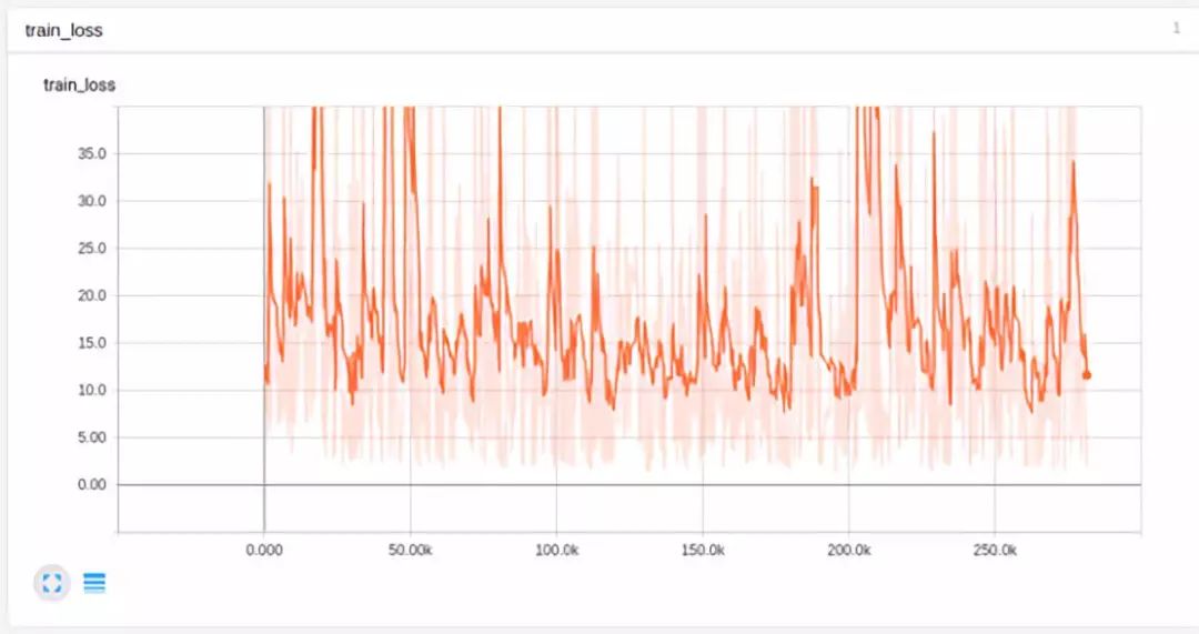
We tried to clip the value range to prevent them from exceeding the limits:

Oh no, look how messy this un-smoothed line is. Is the learning rate too large? We tried decaying the learning rate and training with just one sample point:

You can see the learning rate changed (probably between steps 300 and 3000). Clearly, the learning rate decayed too quickly. So, we slowed down the iteration rate, and the results improved:

You can see we decayed it between steps 2000 and 5000. The results improved, but still not enough, as the loss had not dropped to 0.

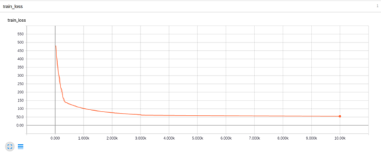
Then we stopped the learning rate decay and tried compressing the values to a smaller range and replaced the tanh function. Although this reduced the loss to 1, we still could not achieve overfitting.

It was at this step that we discovered that after removing batch normalization, the network output quickly became NaN after just one or two iterations. Thus, we stopped batch normalization and changed the initialization to variance scaling. This immediately solved the problem, and we could achieve overfitting with just one or two input samples. Although the values on the Y-axis were clipped below, the initial error was above 5, indicating an error drop of nearly four orders of magnitude.

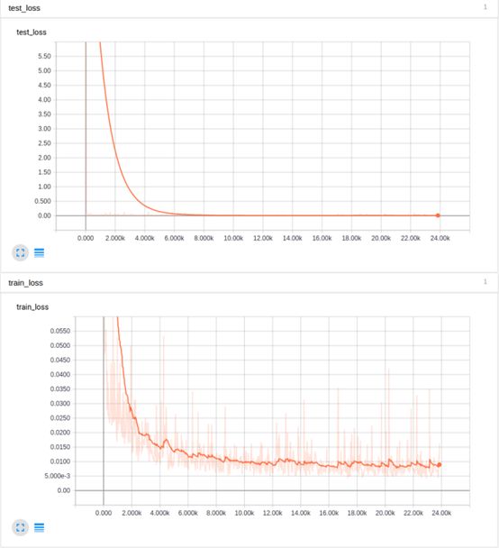
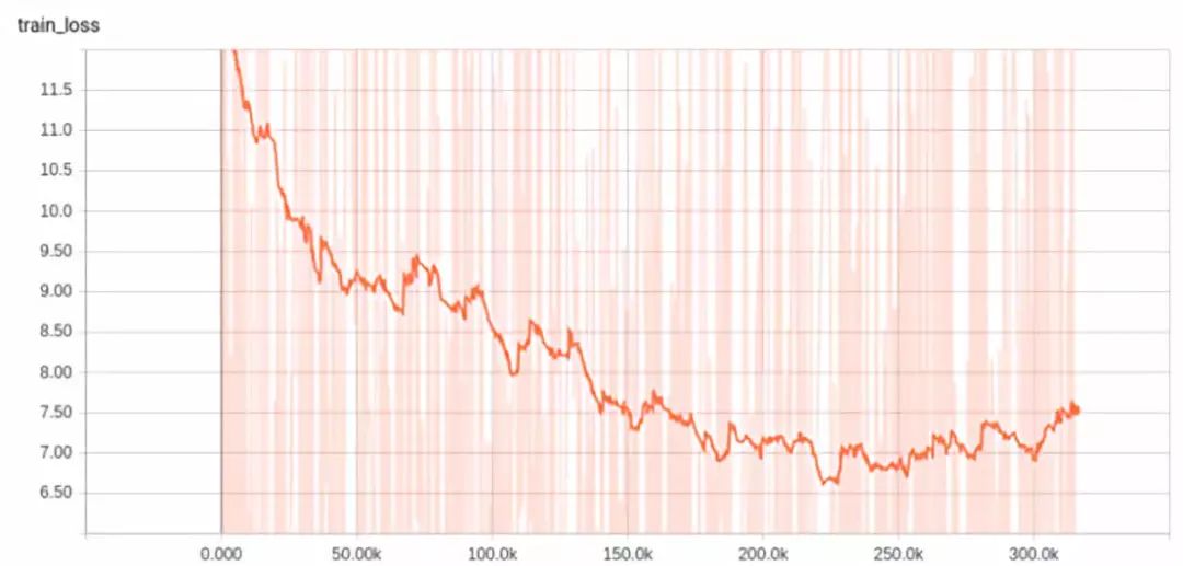
The upper part of the above graph is smoothed, but you can still see that overfitting was quickly reached for the test data, and the loss for the entire training set dropped below 0.01. At this point, we had not yet decayed the learning rate. After reducing the learning rate by an order of magnitude and continuing to train the neural network, we obtained even better results:

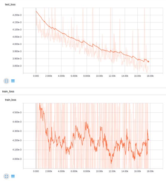
These results are much better! But what if we decayed the learning rate geometrically instead of splitting the training into two parts?

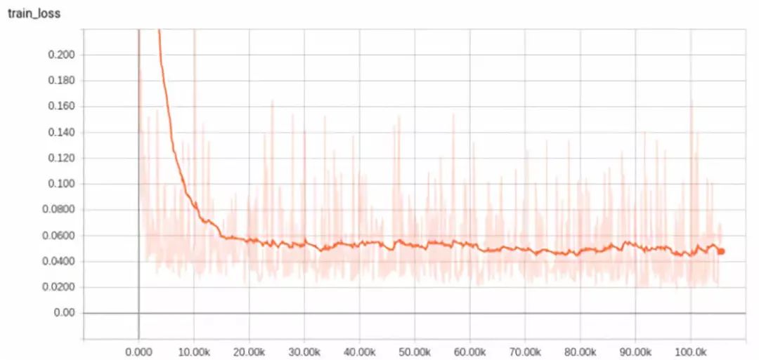
If we multiplied the learning rate by 0.9995 at each iteration, the results would not be so good:

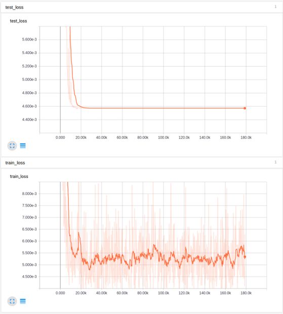
The reason is likely that the learning rate decayed too quickly. Using 0.999995 would be slightly better, but the results were almost the same as having no decay at all. From this series of experiments, we concluded that batch normalization masked the gradient explosion caused by improper initialization, and other than the learning rate decay in the final stages, decaying the learning rate is not very useful for the ADAM optimizer. Alongside batch normalization, clipping value ranges merely masked the real problems. We also transformed our high-variance input data using the tanh activation function.

I hope these basic tips can help you in learning deep neural networks. Often, simple details can have a significant impact.

Related Report:

https://pcc.cs.byu.edu/2017/10/02/practical-advice-for-building-deep-neural-networks/

Countdown to Course Opening in 2 Days

Data Science Bootcamp Session 6

Outstanding Teaching Assistant Recommendation | Jiang Jiang

As a newbie whose understanding of data analysis was limited to Excel, I once thought that analyzing data through coding was incredibly sophisticated. However, I actually achieved it in the Data Science Bootcamp!

The hands-on teaching approach, along with enthusiastic discussions with teaching assistants and classmates, made me gradually feel that each line of code was so approachable. When I realized my thoughts through code and saw the results, it was incredibly exciting!

After practicing with cases from Kaggle and Tianchi, I became very interested in these data competitions. Are there any friends interested in playing together?

As a teaching assistant for the sixth session in North America, I would like to say to all students: High energy ahead, please prepare enough time. If you can submit your homework on time, you will definitely undergo a transformation by the end of the course.