Click on the above “Beginner’s Visual Learning” to add “Star” or “Pin“
Heavyweight content delivered promptly.
1 Motivation and Background
Every day, millions of people use public transport such as subways and civil aviation, making the safety inspection of luggage vital to protect public places from terrorism and other threats, playing an important role in security prevention. However, with the increasing urban population and more people using public transport, the convenience comes with significant insecurity. Therefore, it is crucial to design a system that can help speed up the security check process and improve its efficiency. Deep learning algorithms, such as convolutional neural networks, have been continuously developed and have played a significant role in various fields, including machine translation and image processing. As a fundamental computer vision problem, target detection provides valuable information for image and video understanding and is related to image classification, robotics, facial recognition, and autonomous driving.In this project, we will explore several deep learning-based target detection models to locate and classify prohibited items in X-ray images and compare the performance of these models across different metrics.
Regarding existing research in this field, R. Girshick et al. [29] developed a region-based target detection network (R-CNN) that uses a selective search algorithm to find bounding boxes around objects of interest, but this model is slow to train. A few months later, R. Girshick et al. [30] improved the R-CNN model by enhancing the selective search algorithm, reducing training time, and named the model Fast R-CNN. A year later, K. He, R. Girshick et al. [31] eliminated the selective search algorithm and introduced the Region Proposal Network (RPN), designing a new target detection model called Faster R-CNN, which significantly reduced training time. In 2017, K. He et al. [32] proposed Mask R-CNN, which not only uses bounding boxes to locate objects but also locates the precise pixels of each object.
Unlike the aforementioned region proposal-based methods, some studies introduced another method called regression/classification-based target detection method. D. Erhan et al. [33] launched MultiBox in 2014; J. Redmon et al. [34] invented YOLO in 2016, achieving high detection speeds; subsequently, J. Redmon and A. Farhadi [35] designed a faster model called YOLO v2; in 2016, another research team led by W. Liu et al. [36] introduced a new architecture called SSD network, which has similar accuracy to Faster R-CNN but shorter training time. In our project, we have explored all these region proposal-based frameworks and regression/classification-based frameworks.
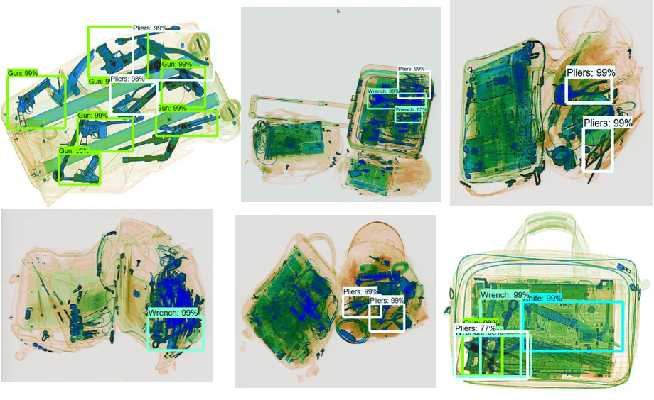
Dataset: The SIXray dataset consists of X-ray images from the Beijing subway. https://github.com/MeioJane/SIXray
2 Problem Statement
The goal of this project is to identify the best algorithm for detecting prohibited items in X-ray images by selecting various algorithms and training multiple models to compare their performance. The prohibited items include guns, knives, wrenches, pliers, and scissors, but hammers are not included in this project due to the scarcity of images in that category. The performance of the models is described by mAP (mean Average Precision), accuracy, and recall, and we will discuss the challenges associated with addressing this problem.
2.1 Algorithms (Target Detection vs. Image Classification)
In image classification, CNN is used as a feature extractor, directly extracting features from all pixels in the image. These features are then used to classify prohibited items in X-ray images. However, this method is computationally expensive and brings a lot of redundant information. Furthermore, standard CNNs include fully connected layers with fixed outputs (i.e., the output of the classification network has a fixed dimension). However, in our dataset, an image may contain many prohibited items of the same or different categories, and these prohibited items may have different spatial locations and aspect ratios. Therefore, using classification methods leads to high computational costs and consumes a lot of time. Thus, we conclude that this dataset is very suitable for target detection algorithms, as the goal of target detection is not only to classify prohibited items but also to locate them by creating bounding boxes.
2.2 Dataset Imbalance
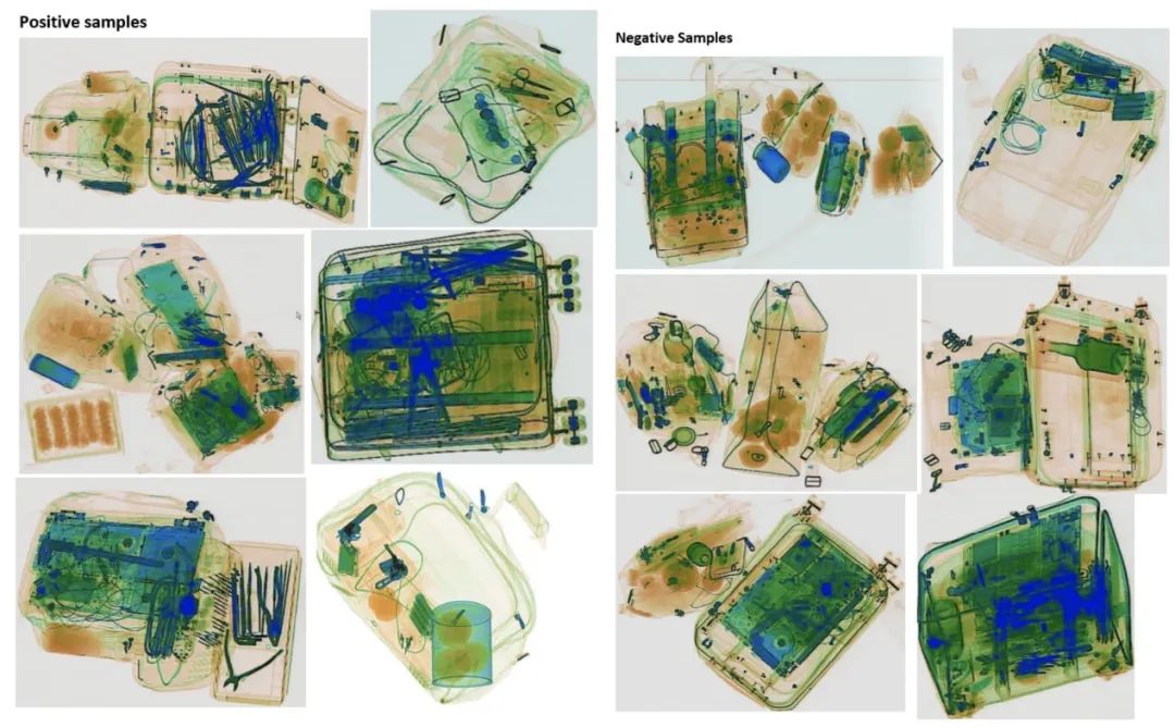
Our dataset is highly imbalanced, with negative samples far outnumbering positive samples. Negative samples mean images that do not contain our objects of interest, while positive samples mean images that contain our objects of interest. In this case, the targets we try to detect in X-ray images are prohibited items such as knives, guns, wrenches, pliers, and scissors.The benefit of using target detection models instead of classification models is that we can train enough positive samples without needing to incorporate negative samples (images) into the training set, as negative samples are implicitly present in the images. All areas in an image that do not relate to the bounding box (the true bounding box of the target) are negative samples. Therefore, due to the imbalanced dataset, we can save time and costs in training large datasets without sacrificing much accuracy.
2.3 Complex Images
Our X-ray image dataset not only consists of the dataset, but also includes unclear images within the imbalanced dataset. Essentially, the luggage images that security checks often deal with contain items that cluster, overlap, and stack randomly with other items. For example, normal items and prohibited items are often mixed in various ways, leading to significant detection issues, such as false detections or missed detections using simple metal detectors or personnel checks.However, by carefully selecting suitable target detection models, we can not only correctly classify prohibited items but also determine their locations in the images, addressing this challenging problem. In the next section, we will introduce the target detection architectures behind each model selected for the project.
3 Data Processing Steps
3.1 Data Acquisition
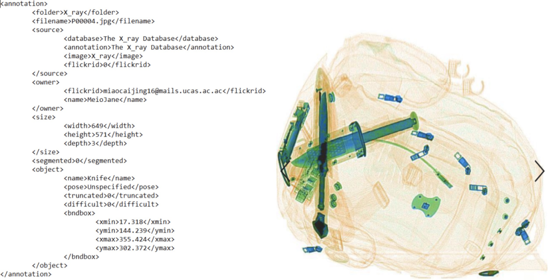
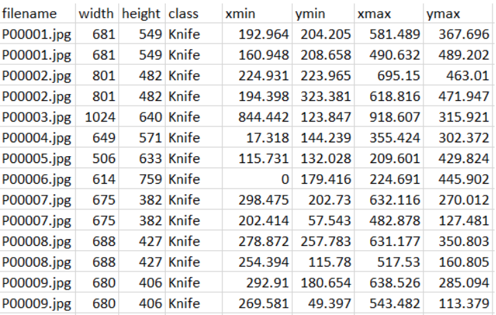
The dataset consists of positive samples (images containing the objects of interest, i.e., the prohibited items we want to locate and classify) and negative samples (images containing non-prohibited items) from the SIXray dataset, which are subsequently used to train and evaluate our models. Additionally, all image label files are located in three separate folders. The position annotation files for our objects of interest are in XML format.
3.2 Preprocessing Images and Label Files to Create Training Data
We use a subset of positive samples for training, and another subset combined with negative samples for testing and evaluation. Due to computational cost and feature capabilities, we did not use the entire SIXray dataset in this project. Our dataset has three main preprocessing steps:
The first step: Obtain the correct labels for each image we want to use. Since we are using a subset of the dataset, new labels need to be retrieved for each image from the dataset, and these labels are later used to test and evaluate our trained model.
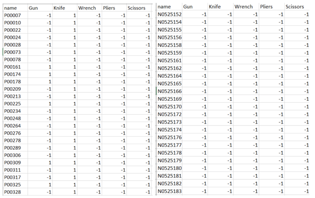
The second step: Create a readable dataset by converting the labeled XML files (which contain metadata for each image, such as category and object location).
The third step: Convert the images and annotation files of positive samples into TensorFlow Record for training the target detection model.
3.3 Creating Training and Training Models
Our training is completed using the TensorFlow Object Detection API, which we can download and install from the link below, and we can also download configuration files and pre-trained target detection models from TensorFlow Model Zoo. Additionally, we tried classification models, but the results were poor, so we switched to using target detection models.
TensorFlow Object Detection API:
https://github.com/tensorflow/models/tree/master/research/object_detection
TensorFlow Object Detection Model Zoo:
https://github.com/tensorflow/models/blob/master/research/object_detection/g3doc/detection_model_zoo.md
TensorFlow Object Detection Configuration for Each Model:
https://github.com/tensorflow/models/tree/master/research/object_detection/samples/configs
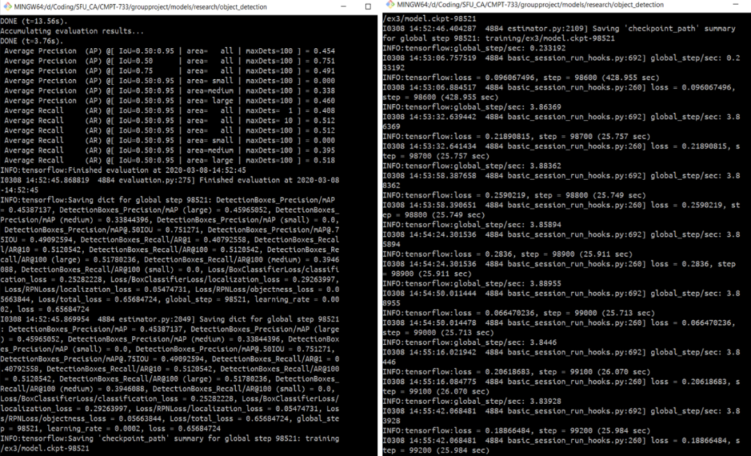
Training was conducted on the Google Cloud Platform with deep learning VM. We trained eight different target detection models.

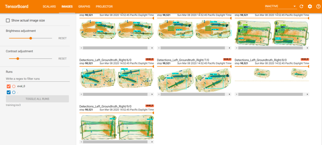
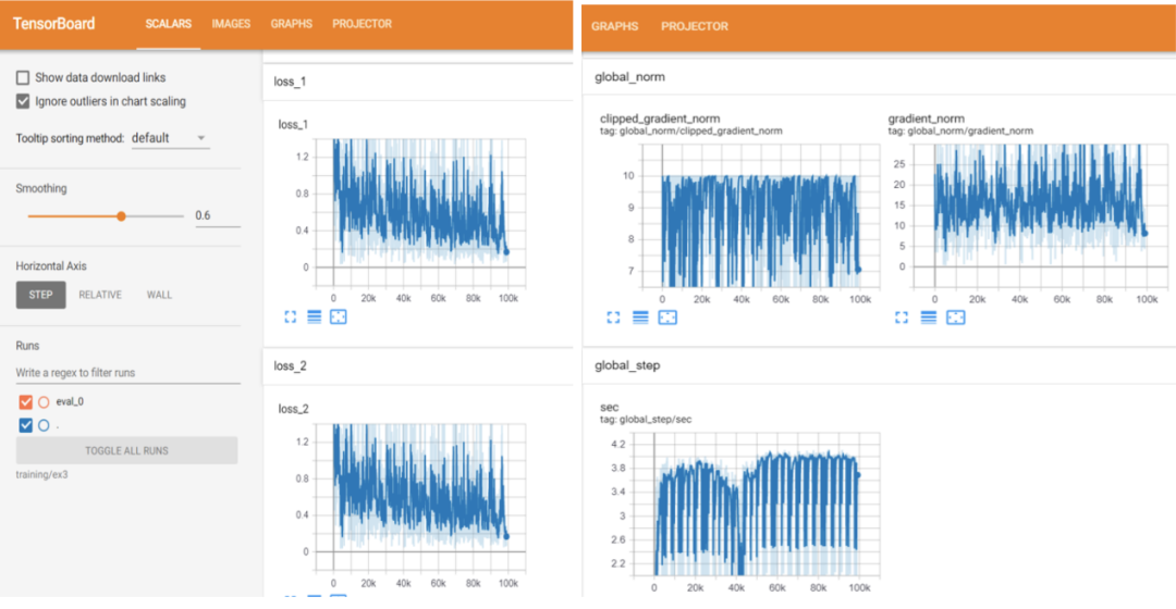
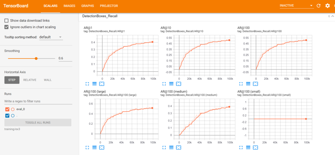
The images used for training consisted of 7200 positive samples. In this project, we did not add negative samples to our training set because the detection model will consider regions of images that do not belong to the true bounding boxes as negative samples. Furthermore, the training process is monitored by TensorBoard, allowing us to view the training progress online, including the number of training steps completed, training loss, validation loss, and more.
3.4 Evaluating Each Model with Different Ratios of Positive-Negative Image Sets
We created an inference graph for the trained model and evaluated it using another subset of positive samples and all negative samples. The performance of the evaluation is measured using Precision-Recall scores and mAP.
Three Test Set Ratios for Model Evaluation:
1. 1800 positive samples + 50,000 negative samples
2. 1800 positive samples + 100,000 negative samples
3. 1800 positive samples + 150,000 negative samples
4 Methods
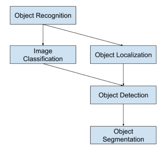
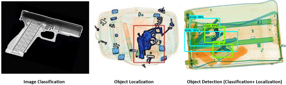
For image classification problems, images serve as inputs, and the model classifies the objects contained in the image. However, the localization problem is to locate the position of objects in the image, but merely locating does not help us predict the object category in the image. Target detection specifies the position of objects in the image and predicts the category of the object. Therefore, in this project, target detection models are very suitable for our X-ray image dataset.
In our project, we implemented eight target detection models with different architectures (described in the next section):
1. SSD Mobilenet_v1
2. SSD Mobilenet_v1_fpn
3. SSD Inception_v2
4. SSD Resnet50
5. R-FCN Resnet101
6. Faster R-CNN Resnet50
7. Faster R-CNN Resnet101
8. Faster R-CNN Inception_v2
4.1 Target Detection Architecture
(1) SSD (Single Shot MultiBox Detector)
Paper Link: https://arxiv.org/abs/1512.02325
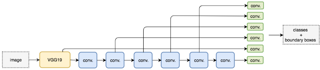
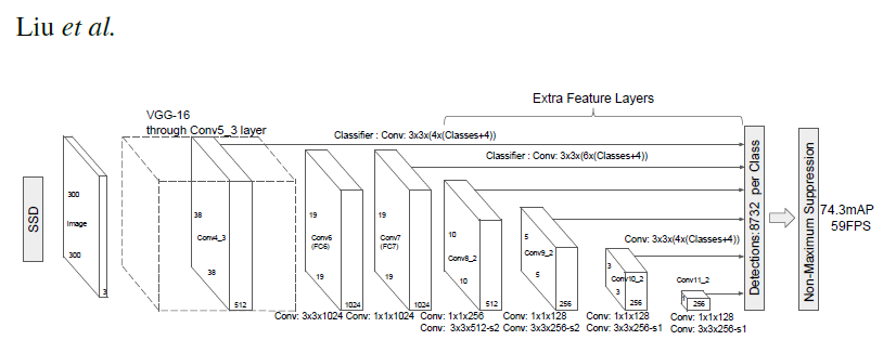
SSD is a method for detecting objects in images using a single deep neural network, which discretizes the output space of bounding boxes into a set of default boxes. These default boxes have different aspect ratios and scales at each feature map location. During prediction, the network generates scores for all object classes present for each default box and adjusts the default boxes to better match the shape of the object.
Compared to other methods that require region proposals, SSD is simpler because it encapsulates all computations within a single network. SSD uses VGG16 as a feature extractor (equivalent to CNN in Faster R-CNN), making SSD easy to train, fast to detect, and directly integrable into systems requiring real-time detection. SSD adopts a feature pyramid hierarchy with fast detection speed, but it performs poorly in detecting small objects because it misses the opportunity to use high-resolution feature maps (e.g., SSD only uses upper feature maps for detection), as shown in the figure below:
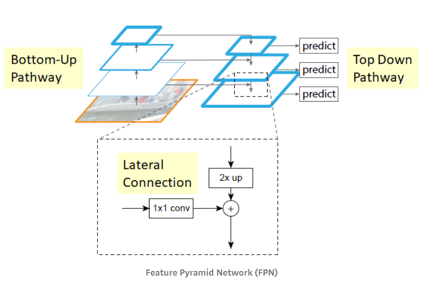
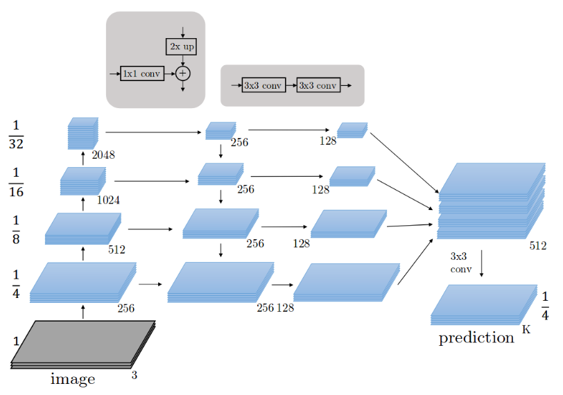
(2) FPN (Feature Pyramid Network)
Paper Link: https://arxiv.org/abs/1612.03144
FPN contains two main paths: a top-down path (semantic strong, low-resolution features) and a bottom-up path (semantic weak, high-resolution features). In addition, the network adds lateral connections that connect the reconstructed layers and corresponding feature maps to help the detector better predict target locations. The entire feature pyramid has rich semantics across all layers and can be quickly constructed without sacrificing feature representation, speed, or memory.
In summary, FPN is a feature extractor designed to build high-level semantic feature maps at various scales (the pyramid concept). FPN is an improvement over multi-scale feature extractors and contains higher quality information compared to feature extractors in other target detection models, such as Faster R-CNN.
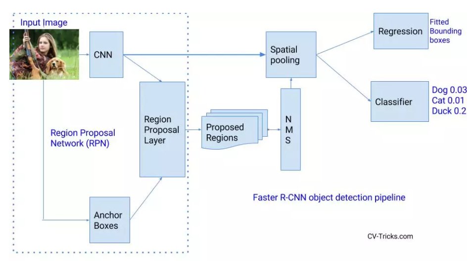
(3) Faster R-CNN (Region-based Convolutional Network)
Paper Link: https://arxiv.org/abs/1506.01497
In simple target detection algorithms, a CNN model is applied to a single image to detect the objects of interest. Since our objects of interest may be located anywhere in the image, we retrain the network by applying different sliding windows to different regions multiple times, which is computationally expensive and very time-consuming. Therefore, we need to attempt to reduce the number of sliding windows.
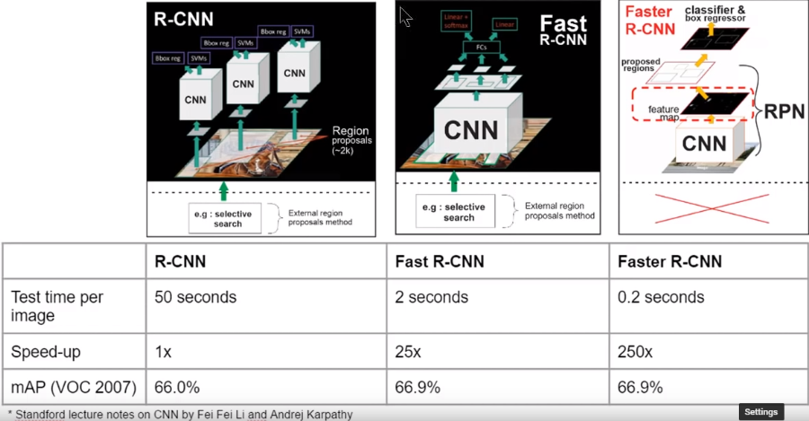
R-CNN: Proposed by Ross Girshick, R-CNN uses a selective search algorithm to extract 2000 region proposals (candidate regions) for each image. The selective search algorithm uses local cues (such as texture, color, etc.) to generate all possible locations of objects, and CNN acts as a feature extractor for each candidate region. Finally, a linear SVM classifier classifies the potential targets in the candidate regions. However, training R-CNN remains computationally expensive because each image still contains about 2000 candidate regions.
Fast R-CNN: Later, the same researcher (Ross Girshick) designed an upgraded version of this model (R-CNN), called Fast R-CNN, which uses a very similar method, such as using a slightly modified selective search method. It does not need to generate 2000 fixed region proposals but extracts a set of region proposals through two main operations: The first operation is CNN model feature extraction, outputting convolutional feature maps (global feature); the second operation uses the Region of Interest (ROI) pooling layer to identify region proposals from the output of the first operation and extract features. This method reduces the computational load.
Faster R-CNN: However, the selective search method remains a very time-consuming operation; thus, a new model called Faster R-CNN was proposed. It does not use the selective search algorithm but introduces a new network to generate region proposals, making Faster R-CNN faster than R-CNN and Fast R-CNN.
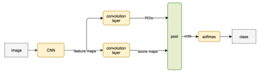
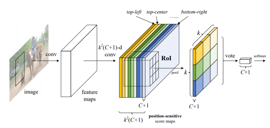
(4) R-FCN (Region-based Fully Convolutional Network)
Paper Link: https://arxiv.org/abs/1605.06409
Compared to previous region-based detectors (such as R-CNN, Fast R-CNN, and Faster R-CNN) that apply expensive region subnetworks hundreds of times, the authors of this paper proposed a new region-based model called R-FCN, which has a fully convolutional architecture that shares all computations almost across the entire image. The authors proposed position-sensitive score maps to address the dilemma between translation invariance in image classification and translation variance in target detection. Thus, this method can adopt fully convolutional image classification backbone (e.g., the latest residual networks ResNet) for target detection.
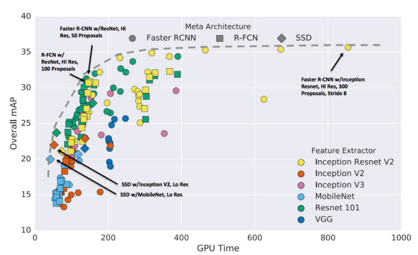
(5) Comparison of Accuracy and Speed Between Models
4.2 Key Features of the Backbone Networks of Target Detection Models
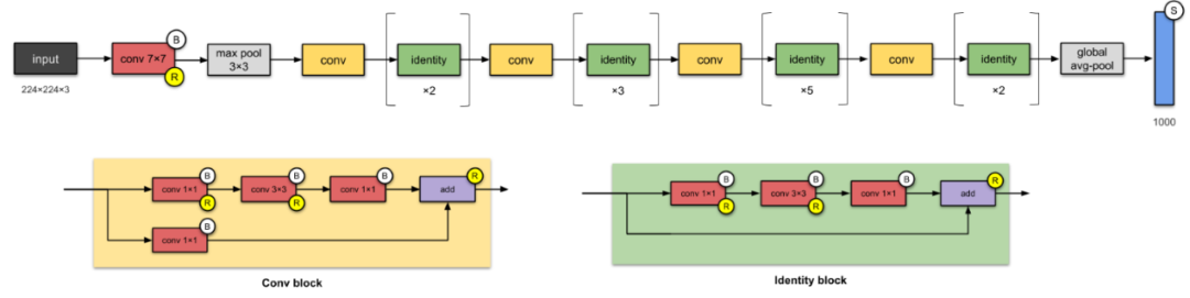
(1) ResNet50 and ResNet101
Paper Link: https://arxiv.org/abs/1512.03385
ResNet is a very deep network with many layers, and it is the first network to use skip connections to solve the gradient vanishing problem caused by deepening the network, which leads to a decrease in accuracy. It also applies batch normalization techniques; note that ResNet101 is a deeper network than ResNet50.
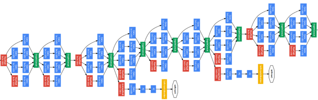
(2) Inception v2
Paper Link: https://arxiv.org/pdf/1512.00567v3.pdf
The Inception_v2 architecture contains three main components: first, it introduces two additional auxiliary classifiers in the middle of the network to address the gradient vanishing problem; second, due to different filter sizes in the same layer, it has a deeper and wider network compared to ResNet (structure); finally, to address the information loss caused by reducing input size, the network upgraded Inception_v1 by using two 3×3 convolutions (instead of one 5×5 convolution).
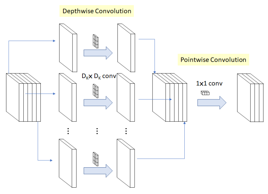
(3) MobileNet v2
Paper Link: https://arxiv.org/abs/1704.04861
The key to MobileNet is that it uses depthwise separable convolutions to build lightweight deep networks. This means that the network applies depthwise convolutions before applying pointwise convolutions. Standard convolutions can filter and merge through a single operation, but depthwise separable convolutions are done in two separate steps, thereby speeding up computation.
(4) Comparison of Accuracy and Speed Between Models
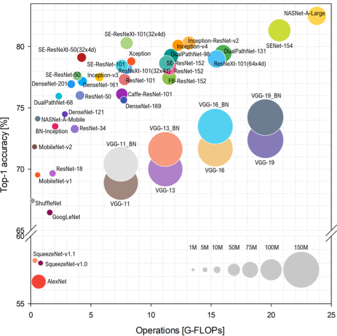
Note:
1. Complexity can be represented by floating-point operations or the number of triggers required to find a solution, meaning triggers are the basic units of computation, and the number of triggers indicates the cost of executing a series of operations.
2. Inception v3 has the same architecture as Inception v2 but with some minor changes.
From the above figure, in terms of computation time, we can rank the models used from fastest to slowest as follows: ResNet101, Inception_v3, ResNet50, and MobileNet_v1. On the other hand, in terms of accuracy from highest to lowest, the order is Inception_v3, ResNet101, ResNet50, and MobileNet_v1.
5 Evaluation
The target detection model includes two main tasks: the first task is the classification task, which determines whether the image contains our objects of interest; the second task is the localization task, which determines the position of the objects of interest in the image. Additionally, our dataset faces the challenges of a high imbalance between positive and negative samples and irregular distributions of different categories of prohibited items. Therefore, using accuracy measures alone to evaluate the model is insufficient; we also need to assess the likelihood of our model misclassifying objects of interest and non-interest objects. Thus, we evaluate the model scores or confidence scores based on each bounding box surrounding our objects of interest to assess our model’s ability to predict target positions and categories at any acceptable threshold. Average Precision (AP) is a commonly used metric for target detection tasks, and we also need to understand some important concepts, such as Precision-Recall curves, AP, and IoU.
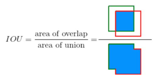
5.1 Intersection over Union (IoU) Threshold
In evaluating whether the target detection model can classify the categories of prohibited items and predict their locations in the image, an important threshold is the Intersection over Union (IoU), which is the ratio of the area of intersection between the ground truth box and our model’s predicted box to the area of their union.
5.2 Precision-Recall Curve
Our project samples and categories are imbalanced, and the precision-recall metric is a very useful measure of successful predictions.
Precision (P) is the number of true positive samples (TP) divided by the sum of true positive samples and false positive samples (FP). [P=TP/(TP+FP)]
Recall (R) is the number of true positive samples (TP) divided by the sum of true positive samples (TP) and false negative samples (FN). [R=TP/(TP+FN)]
To evaluate these metrics, we need to select some thresholds to consider the model’s prediction direction.
True positive samples (TP) are correct predictions where IoU >= threshold.
False positive samples (FP) are incorrect predictions where IoU < threshold.
False negative samples (FN) are missed detections of objects of interest.
True negative samples (TN) are implicit measures of the target detection model; true negative samples are bounding boxes that do not contain our objects of interest, and there are many such bounding boxes in each image. We do not need to explicitly measure true negative samples, as the other measures above can perform similar functions in the opposite direction.
Precision indicates our model’s ability to detect objects of interest, while recall indicates our model’s ability to find all relevant bounding boxes for the objects of interest. From the formulas for precision and recall, it can be seen that precision will not decrease as recall decreases.
The definition of precision TP/(TP+FP) indicates that lowering the model’s threshold may increase the denominator by increasing the number of relevant returned results. If the threshold is set too high, it may increase the number of true positive samples returned, thereby improving precision; whereas if the previous threshold is approximately correct or too low, further lowering the threshold may increase the number of false positive samples, thus reducing precision. The definition of recall R=TP/(TP+FN) indicates that FN does not depend on the selected threshold, meaning that lowering the threshold may improve recall by increasing the number of true positive samples, thus keeping recall unchanged while precision fluctuates. However, selecting the correct threshold is difficult, so we prefer to find all possible thresholds and take their average, which is why average precision (AP) is very important.
Precision and Recall Curve: illustrates the trade-off between precision and recall for different thresholds. The high area under the curve represents high recall and high precision, where high precision is related to low FP, and high recall is related to low FN. Both high scores indicate that our model returned accurate results (high precision) and returned most true positive samples (high recall).
Models with high recall but low precision can locate most bounding boxes around our objects of interest, but most predicted classes of these objects are incorrect compared to the true labels. Conversely, models with high precision but low recall return very few relevant bounding boxes, but most of these bounding boxes’ predicted classes are correct compared to the true labels. In summary, we want models with high precision and high recall because they will return many relevant bounding boxes, all correctly labeled.
5.3 Average Precision (AP) and Mean Average Precision (mAP)
Average Precision (AP) summarizes the precision-recall curve by averaging the precision achieved at each threshold level weighted by the increase in recall at previous thresholds. [AP=∑n(Rn−Rn−1)Pn] where Pn and Rn are the precision and recall at the nth threshold. According to the formula above, AP is the average precision at all recall levels for each threshold.
Mean Average Precision (mAP) is defined as the average of average precision for all different categories; however, there are two different types of mAP: Micro mAP and Macro mAP. Macro mAP independently computes the AP measure for each class of interest and then calculates the average, meaning Macro mAP treats all classes equally; in contrast, Micro mAP aggregates the contributions of all classes to compute the AP metric.
Results:
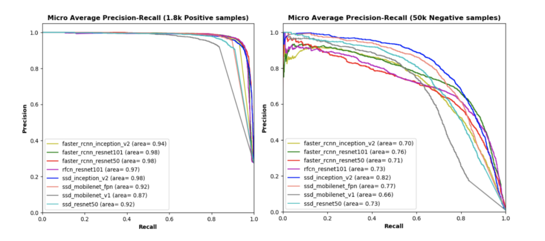
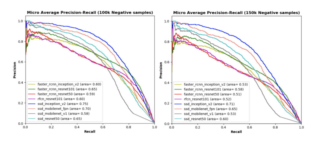
We trained all models with 7200 positive samples while evaluating with another 1800 positive samples and different numbers of negative samples (50,000, 100,000, and 150,000, respectively). The charts above show the precision-recall curves of different models under test datasets with different ratios of positive and negative samples; the larger the area under the curve, the higher the precision and recall at each threshold.
From the charts, we can observe:
(1) In the top left image, testing our model using only 1800 positive samples without any negative samples, although the area under the curve for SSD_Mobilenet_v1 is relatively smaller than other models, all models have a high area under the curve. The remaining three images display the performance of each model when tested using different subsets of the test dataset (i.e., 50,000, 100,000, and 150,000 negative samples);
(2) Compared to other models under each test dataset, the area under the curve for the SSD_Inception_v2 model is the largest. Additionally, in every ratio of positive and negative samples in the test dataset, SSD-based models (e.g., SSD_Mobilenet_v1_fpn and SSD_Resnet50) have larger areas under the curve than other models (e.g., R-FCN and Faster R-CNN), except for SSD_Mobilenet_v1.
(3) In each test dataset, SSD_Mobilenet_v1 has the lowest area under the curve, indicating that the performance of our model depends not only on the detection network but also on the network backend (e.g., different CNN models used for feature extraction).
(4) SSD detection models based on Inception_v2, Mobilenet_v1_fpn, and Resnet50 outperform R-FCN and Faster R-CNN models with similar network backends. In contrast, the SSD model using simple extraction networks (e.g., Mobilenet_v1) performs the worst among all our models.
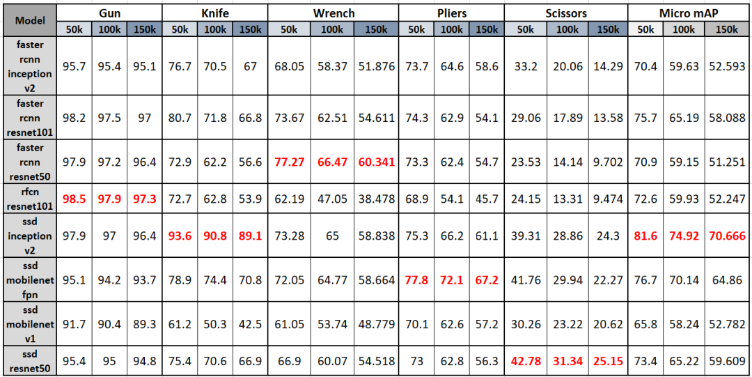
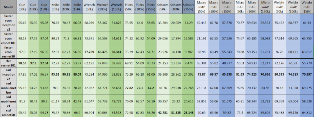
The table shows the average accuracy (AP) of different models in test datasets containing varying proportions of prohibited items, and the last three columns show the mean average precision (mAP) for each model under different proportions of the dataset.
From the table, we can clearly observe:
(1) As more negative samples are added to the test dataset (from 50k to 150k), both AP and mAP decrease accordingly.
(2) For guns, RFCN_Resnet101 performs best, while other models (e.g., Faster_RCNN_Resnet50/101 and SSD_Inception_v2) are very close; for knives, SSD_Inception_v2 has the highest AP and significantly outperforms other models. The best model can achieve an AP of up to 90% for both guns and knives; for wrenches and pliers, Faster_RCNN_Resnet50 and SSD_Mobilenet_v1_fpn achieve the highest AP of 60-80%. However, for scissors, SSD_Resnet50 has the highest AP but only ranges from 20% to 40%, indicating that scissors may be the most challenging prohibited item to detect. Therefore, it is recommended that machine learning engineers modify the model or add more data for the scissors category.
Overall, our project uses Micro mAP to evaluate the overall performance of each model. SSD_Inception_v2 has the highest Micro mAP, which is consistent with our previous analysis of the average recall rate curve.

The line chart above summarizes the last three columns of the table using the Micro mAP scores for each model. SSD_Inception_v2 is the best model in our project, followed by SSD_Mobilenet_v1_fpn, while the performance of SSD_Mobilenet_v1 is the most disappointing among all models.
6 Data Products
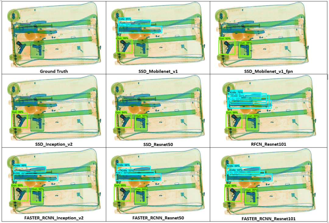
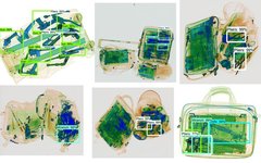
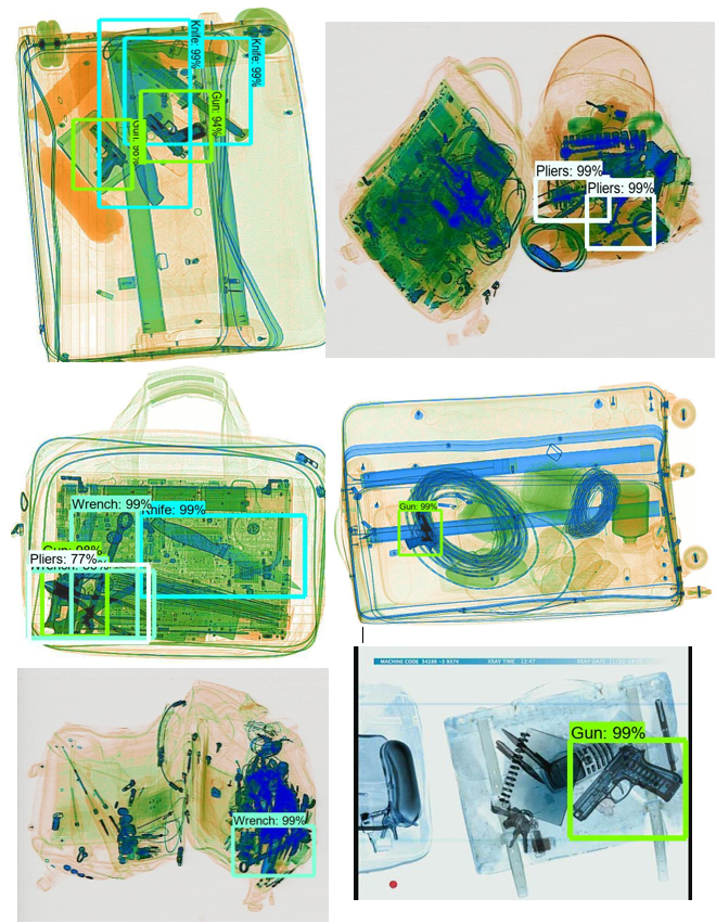
The test images show the performance of the different target detection models we trained and the actual conditions of the images.
In the first test image, we can see that there are four dangerous items in the luggage image, including two guns and three overlapping knives. Among all models, SSD_Mobilenet_v1_fpn, SSD_Inception_v2, and SSD_Resnet50 can only detect the guns while missing all the knives, while the other models can detect both guns and knives simultaneously. RFCN_Resnet101 and Faster_RCNN_Resnet101 perform best compared to other models, although RFCN_Resnet101 places more bounding boxes on the prohibited items, they can detect all four prohibited items with very high accuracy.
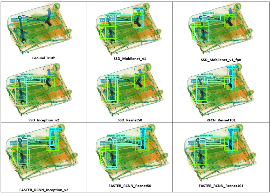
The second test image is more challenging than the previous one, containing three different types of dangerous items: wrenches, guns, and knives. The actual image shows three wrenches, two guns, and one knife scattered and overlapping randomly. SSD_Mobilenet_v1_fpn and SSD_Inception_v2 can detect the wrenches and guns but miss the knives, while all other models, except SSD_Resnet50, can detect all three prohibited items. SSD_Resnet50 can detect the guns and wrenches with very low accuracy scores but misses the knife and wrenches. RFCN_Resnet101, Faster_RCNN_Resnet101, and Faster_RCNN_Resnet50 perform best in this image as they can identify all prohibited items and accurately locate them with high scores.
7 Lessons Learned
The following three points can be learned from this project: how target detection models work; why target detection models are needed; and how to evaluate the performance of target detection models.
(1) Why use target detection instead of classification models? Typically, we choose CNN models to address image classification problems; however, in this project, CNNs could not recognize and locate prohibited items in the X-ray dataset images. For example, we tried VGG16 and ResNet50 models, but the results were disappointing. To explain this phenomenon, we conducted some research on computer vision and found that classification models alone are not suitable for solving the project’s problems. The challenging tasks in this project include feature extraction and multi-target localization. In contrast, we implemented a better alternative method, which is the target detection model.
(2)Different target detection architectures. For example, Faster R-CNN, SSD, R-FCN, and FPN have been explained in detail in the previous sections regarding their structures, functions, and advantages. To implement target detection models, we used the TensorFlow Object Detection API and trained them on the Google Cloud Platform. We trained several models and evaluated their performance.
(3) Model evaluation metrics. In the evaluation section, we learned three new concepts regarding model evaluation metrics, including precision-recall curves, average precision (AP), mean average precision (mAP), and intersection over union (IoU) thresholds. We used AP and Micro mAP as the primary metrics to evaluate all trained target detection models and select the best-performing model.
Future Work:
(1)To improve the accuracy of target detection models, we need to add more ‘positive’ images. In the future, we can also integrate some negative samples into the training set. In particular, it is necessary to add images containing scissors, as recognizing scissors seems to be the most challenging for all our models. The best-performing model for detecting scissors can only achieve 42% accuracy, possibly due to the lack of images of scissors in our dataset, as we only have 983 images containing scissors, which is far below other categories. Our current dataset is imbalanced between positive and negative samples (with 8929 positive images and 1050302 negative images), and the number of images containing prohibited items is also imbalanced across each category. Our project only used positive images to train the models, but positive images account for less than 1%, and some of these images still need to be included in the test dataset. In the future, we can integrate some negative samples into our training dataset.
(2)Making trade-offs between model time and accuracy. Since some applications require real-time target detection, in such cases, models with the highest accuracy but slow training and evaluation speeds may not be suitable.
8 Summary
Project Goal: To find the best algorithm that can correctly classify and accurately locate prohibited items in X-ray images.
Project Dataset: Using a large-scale dataset – the SIXray dataset, which consists of over one million X-ray images containing varying numbers of prohibited and non-prohibited items.
Project Models: Due to the poor performance of classification CNN models, we switched to using target detection models to address this issue; we selected several target detection architectures, such as SSD, Faster R-CNN, FPN, and R-FCN, which have different feature extraction backends, such as CNN models (including ResNet, Inception, and MobileNet); we successfully trained eight target detection models and evaluated the performance of each model, in order to find the best-performing model in our imbalanced dataset, using mean average precision (mAP) to measure the overall performance of each model in predicting different categories of prohibited items. In this project, SSD_Inception_v2 proved to be the most suitable model with the highest mean average precision score.
Future Work: Optimize model performance to enhance the detection of prohibited items like scissors, as the number of images of scissors accounts for only 0.001% of the entire dataset. One possible solution is to increase the quantity of the training dataset by adding more positive samples.
Additional Images:
T
References
1. SIXray Dataset: https://github.com/MeioJane/SIXray
2. SIXray: A Large-scale Security Inspection X-ray Benchmark for Prohibited Item Discovery in Overlapping Images:
https://arxiv.org/pdf/1901.00303.pdf
3. TensorFlow Object Detection API document:
https://github.com/tensorflow/models/tree/master/research/object_detection
4. TensorFlow Object Detection Model Zoo:
https://github.com/tensorflow/models/blob/master/research/object_detection/g3doc/detection_model_zoo.md
5. TensorFlow Object Detection Model Config files:
https://github.com/tensorflow/models/tree/master/research/object_detection/samples/configs
6. Feature Pyramid Network:
https://medium.com/@jonathan_hui/understanding-feature-pyramid-networks-for-object-detection-fpn-45b227b9106c
7. COCO Dataset: http://presentations.cocodataset.org/COCO17-Stuff-FAIR.pdf
8. R-FCN Research paper: https://arxiv.org/abs/1605.06409
9. R-FCN explanation:
https://medium.com/@jonathan_hui/understanding-region-based-fully-convolutional-networks-r-fcn-for-object-detection-828316f07c99
10. ResNet Research paper: https://arxiv.org/abs/1512.03385
11. Inception Research paper: https://arxiv.org/pdf/1512.00567v3.pdf
12. MobileNet Research paper: https://arxiv.org/abs/1704.04861
13. MobileNet explanation:
https://towardsdatascience.com/review-mobilenetv1-depthwise-separable-convolution-light-weight-model-a382df364b69
14. Object Detection metric reviews:
https://blog.zenggyu.com/en/post/2018-12-16/an-introduction-to-evaluation-metrics-for-object-detection/
15. Object Detection metric explanation:
https://medium.com/@timothycarlen/understanding-the-map-evaluation-metric-for-object-detection-a07fe6962cf3
16. Faster R-CNN explanation: https://towardsdatascience.com/review-faster-r-cnn-object-detection-f5685cb30202
17. Introduction to Object Detection:
https://machinelearningmastery.com/object-recognition-with-deep-learning/
18. Object Detection model reviews: https://cv-tricks.com/object-detection/faster-r-cnn-yolo-ssd/
19. History of R-CNN, Fast R-CNN, and Faster R-CNN:
https://towardsdatascience.com/r-cnn-fast-r-cnn-faster-r-cnn-yolo-object-detection-algorithms-36d53571365e
20. Should we integrate Negative samples into training dataset:
https://stats.stackexchange.com/questions/315748/object-detection-how-to-annotate-negative-samples
21. Object Detection metrics: https://github.com/rafaelpadilla/Object-Detection-Metrics
22. Scikit-learn Precision-Recall:
https://scikit-learn.org/0.15/auto_examples/plot_precision_recall.html
23. Mean Average Precision: Micro vs Macro:
https://datascience.stackexchange.com/questions/15989/micro-average-vs-macro-average-performance-in-a-multiclass-classification-settin
24. Mean Average Precision: https://medium.com/@jonathan_hui/map-mean-average-precision-for-object-detection-45c121a31173
25. Benchmark Analysis of Representative Deep Neural Network Architectures:
https://arxiv.org/pdf/1810.00736.pdf
26. Flop Definition:
https://www.stat.cmu.edu/~ryantibs/convexopt-S15/scribes/09-num-lin-alg-scribed.pdf
27. Object Detection speed and accuracy comparison:
https://mc.ai/object-detection-speed-and-accuracy-comparison-faster-r-cnn-r-fcn-ssd-and-yolo/
28. Single Shot Detection (SSD):
https://medium.com/@jonathan_hui/what-do-we-learn-from-single-shot-object-detectors-ssd-yolo-fpn-focal-loss-3888677c5f4d
29. R. Girshick, J. Donahue, T. Darrell, and J. Malik, “Rich feature hierarchies for accurate object detection and semantic segmentation,” in CVPR, 2014
30. R. Girshick, “Fast R-CNN,” in ICCV, 2015
31. Ren, K. He, R. Girshick, and J. Sun, “Faster R-CNN: Towards real-time object detection with region proposal networks,” in NIPS, 2015, pp. 91–99.
32. K. He, G. Gkioxari, P. Dollár, and R. B. Girshick, “Mask R-CNN,” in ICCV, 2017
33. D. Erhan, C. Szegedy, A. Toshev, and D. Anguelov, “Scalable object detection using deep neural networks,” in CVPR, 2014
34. Redmon, S. Divvala, R. Girshick, and A. Farhadi, “You only look once: Unified, real-time object detection,” in CVPR, 2016
35. J. Redmon and A. Farhadi, “YOLO9000: better, faster, stronger,” arXiv:1612.08242, 2016
36. W. Liu, D. Anguelov, D. Erhan, C. Szegedy, S. Reed, C.-Y. Fu, and A. C. Berg, “SSD: Single Shot Multibox Detector,” in ECCV, 2016.
 End
End 
Exchange Group
Welcome to join the WeChat group of our public account to communicate with peers. Currently, there are WeChat groups for SLAM, 3D vision, sensors, autonomous driving, computational photography, detection, segmentation, recognition, medical imaging, GAN, algorithm competitions, etc. (which will gradually be subdivided). Please scan the WeChat number below to join the group, and note: “nickname + school/company + research direction”, for example: “Zhang San + Shanghai Jiao Tong University + Visual SLAM”. Please follow the format for notes, otherwise, you will not be approved. After successful addition, you will be invited to relevant WeChat groups based on your research direction. Please do not send advertisements in the group, otherwise, you will be removed from the group. Thank you for your understanding~