Summary of XGBoost Parameter Tuning

XGBoost has shone in Kaggle competitions. In previous articles, the principles of the XGBoost algorithm and the XGBoost splitting algorithm were introduced. Most explanations of XGBoost parameters online only scratch the surface, making it extremely unfriendly for those new to machine learning algorithms. This article will explain some important parameters while referring to mathematical formulas to enhance understanding of the principles of the XGBoost algorithm and will illustrate the parameter tuning ideas of XGBoost through classification examples.

The framework and examples in this article are derived from the translation of https://www.analyticsvidhya.com/blog/2016/03/complete-guide-parameter-tuning-xgboost-with-codes-python/ and the content and code have been modified based on personal understanding. The examples in this article only handle training data and use five-fold cross-validation rate as the standard for measuring model performance.

Code link: https://github.com/zhangleiszu/xgboost-

Table of Contents

1. Simple Review of XGBoost Algorithm Principles

2. Advantages of XGBoost

3. Explanation of XGBoost Parameters

4. Parameter Tuning Example

5. Summary

1. Simple Review of XGBoost Algorithm Principles

Each tree in the XGBoost algorithm fits the second-order derivative expansion of the loss function of the previous model, and then combines multiple trees to provide classification or regression results. Therefore, as long as we understand the construction process of each tree, we can well understand the principles of the XGBoost algorithm.

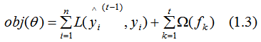
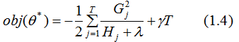
Assuming that the prediction results for the first t-1 trees are , the true result is y, and let L represent the loss function, then the current model’s loss function is:

The XGBoost method constructs trees while considering regularization, defining the complexity of each tree as:

Therefore, the loss function including the regularization term is:

Minimizing (1.3) yields the final objective function:

The objective function is also called the scoring function, which is a standard for measuring the quality of the tree structure; the smaller the value, the better the structure of the tree. Therefore, the node splitting rule of the tree is to choose the point where the objective function value decreases the most as the splitting point.

As shown in the figure below, the difference in the objective function before and after splitting a certain node is referred to as Gain.

Choosing the splitting point with the greatest Gain decrease leads to tree splits; this process continues until a complete tree is formed.

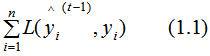
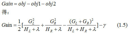
Thus, as long as we know the parameter values in (1.5), we can basically determine the tree model, where represents the sum of the second derivatives of the loss function for the left child node, represents the sum of the second derivatives of the loss function for the right child node, represents the sum of the first derivatives of the loss function for the left child node, represents the sum of the first derivatives of the loss function for the right child node. 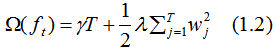represents the regularization coefficient, represents the difficulty of splitting nodes, and and define the complexity of the tree. To simplify, once we have set the loss function L, the regularization coefficient and the difficulty of splitting nodes , the tree model can basically be determined. The three parameters are key considerations for XGBoost parameter selection.

2. Advantages of XGBoost

1. Regularization

XGBoost considers the regularization term when splitting nodes (as shown in Figure 1.3), which reduces overfitting. In fact, XGBoost is also known as “regularized boosting” technology.

2. Parallel Processing

Although XGBoost generates each decision tree in a serial manner, we can achieve parallel processing when splitting nodes, thus XGBoost supports implementation on Hadoop.

3. High Flexibility

XGBoost supports custom objective functions and evaluation functions. The evaluation function is the standard for measuring the quality of the model, while the objective function is the loss function. As discussed in the previous section, as long as we know the loss function and then calculate its first and second derivatives, we can determine the splitting rules for the nodes.

4. Missing Value Handling

XGBoost has built-in rules for handling missing values during node splits. Users need to provide a value that is different from other samples (e.g., -999), and then use this value as the missing value parameter.

5. Built-in Cross-Validation

XGBoost allows the use of cross-validation in each iteration, making it easy to obtain the cross-validation rate and determine the optimal boosting iteration count without needing traditional grid search methods to find the best iteration count.

6. Continue from Existing Models

XGBoost can continue training from the results of the previous round, thus saving runtime. This can be achieved by setting the model parameter “process_type” = update.

3. Explanation of XGBoost Parameters

XGBoost parameters are divided into three categories:

1. General Parameters: Control the macro functions of the model.

2. Booster Parameters: Control the generation of trees in each iteration.

3. Learning Objective Parameters: Determine the learning scenario, such as the loss function and evaluation function.

3.1 General Parameters

• booster [default = gbtree]

The available models are gbtree and gblinear. gbtree uses tree-based models for boosting, while gblinear uses linear models for boosting, with gbtree as the default. Here we only introduce tree booster, as its performance far exceeds that of linear booster.

• silent [default = 0]

  When set to 0, it prints runtime information; when set to 1, it does not print runtime information.

• nthread

  Number of threads during XGBoost runtime, default is the maximum number of threads that can run on the current system.

• num_pbuffer

  Buffer size for prediction data, usually set to the size of the training samples. The buffer retains the prediction results after the last iteration, automatically set by the system.

• num_feature

  Sets the feature dimension to construct the tree model, automatically set by the system.

3.2 Booster Parameters

• eta [default = 0.3]

Controls the weight of the tree model, similar in meaning to the learning rate in the AdaBoost algorithm. It reduces the weight to avoid overfitting. When optimizing eta, it needs to be considered together with the number of iterations (num_boosting_rounding). For example, if the learning rate is reduced, the maximum number of iterations should be increased; conversely, if the learning rate is increased, the maximum number of iterations should be decreased.

Range: [0,1]

Model iteration formula:

Where represents the output result of the first t trees combined with the model, represents the t-th tree model, α represents the learning rate, controlling the weight of model updates.

• gamma [default = 0]

Controls the minimum loss function value for splitting nodes, corresponding to γ in (1.5). If γ is set too high (i.e., (1.5) is less than zero), then no node splitting occurs, thereby reducing the complexity of the model.

• lambda [default = 1]

Represents the L2 regularization parameter, corresponding to λ in (1.5). Increasing the value of λ makes the model more conservative, avoiding overfitting.

• alpha [default = 0]

Represents the L1 regularization parameter. The significance of L1 regularization lies in dimensionality reduction. Increasing the alpha value makes the model more conservative, avoiding overfitting.

Range: [0,∞]

• max_depth [default=6]

Represents the maximum depth of the tree. Increasing the depth of the tree raises its complexity, which may lead to overfitting; 0 indicates no limit on the maximum depth of the tree.

Range: [0,∞]

• min_child_weight [default=1]

Represents the minimum sum of sample weights for leaf nodes, which differs from the previously introduced min_child_leaf parameter. min_child_weight refers to the sum of sample weights, whereas min_child_leaf refers to the total number of samples.

Range: [0,∞]

• subsample [default=1]

  Represents the random sampling of a certain proportion of samples to construct each tree. Reducing the proportion parameter subsample value makes the algorithm more conservative, avoiding overfitting.

  Range: [0,1]

• colsample_bytree, colsample_bylevel, colsample_bynode

  These three parameters represent random sampling of features and have a cumulative effect.

  colsample_bytree represents the proportion of features split for each tree.

  colsample_bylevel represents the proportion of features split for each level of the tree.

  colsample_bynode represents the proportion of features split for each node of the tree.

  For example, if there are 64 features in total, setting {‘colsample_bytree’ : 0.5 , ‘colsample_bylevel’ : 0.5 , ‘colsample_bynode’ : 0.5 } means that 4 features are randomly sampled for splitting at each node of the tree.

  Range: [0,1]

• tree_method string [default = auto ]

  Indicates the method for constructing the tree, specifically the algorithm for selecting split points, including greedy algorithm, approximate greedy algorithm, histogram algorithm.

  exact: greedy algorithm

  aprrox: approximate greedy algorithm, selecting quantiles of features for splitting.

  hist: histogram splitting algorithm, which is also used by the LightGBM algorithm.

• scale_pos_weight [default = 1]

  When there is an imbalance between positive and negative samples, setting this parameter to a positive value can accelerate algorithm convergence.

  Typical values can be set as: (number of negative samples)/(number of positive samples).

• process_type [default = default]

  default: normal boosting tree construction process.

  update: build boosting trees from existing models.

3.3 Learning Task Parameters

Parameters are set according to the task and purpose.

objective, training objective, classification or regression.

reg : linear, linear regression.

reg : logistic, logistic regression.

binary : logistic, using LR for binary classification, outputting probabilities.

binary : logitraw, using LR for binary classification, outputting classification scores before logistic transformation.

eval_metric, metrics for evaluating the validation set, default is set according to the objective function. By default, mean squared error is used for regression, error rate for classification, and average precision for ranking.

rmse: root mean square error.

mae: mean absolute error.

error: error rate.

logloss: negative log loss.

auc: area under the ROC curve.

seed [default=0]

Random seed; setting it allows for the reproduction of random data results.

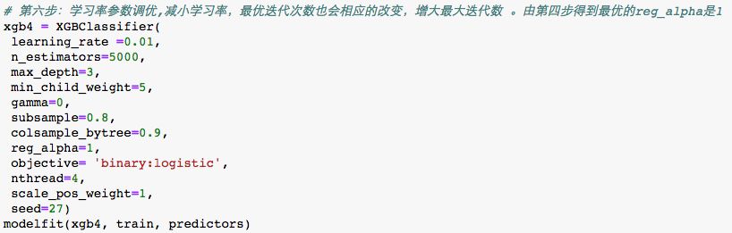
4. Parameter Tuning Example

The original dataset and the dataset processed through feature engineering can be downloaded from the links at the beginning. The algorithm is developed in the Jupyter Notebook interactive interface.

Define the model evaluation function and obtain the optimal number of iterations based on a certain learning rate. The function definition is as follows:

Step1:

Set default parameters based on experience; the optimal number of iterations obtained by calling the modelfit function is 198.

Step2: Tuning Maximum Tree Depth and Minimum Leaf Node Weight

Based on the optimal number of iterations obtained in the first step, update the model parameter n_estimators, then call the GridSearchCV class for cross-validation model setup, and finally call the fit function of the XGBClassifier class to obtain the optimal maximum tree depth and minimum leaf node weight.

a) Set the range for maximum tree depth and minimum leaf node weight:

b) Set up cross-validation model using GridSearchCV:

c) Update parameters using the fit function of the XGBClassifier class:

Step3: Tuning the gamma parameter

Step4: Tuning the subsample and colsample_bytree parameters

Step5: Tuning the regularization parameters

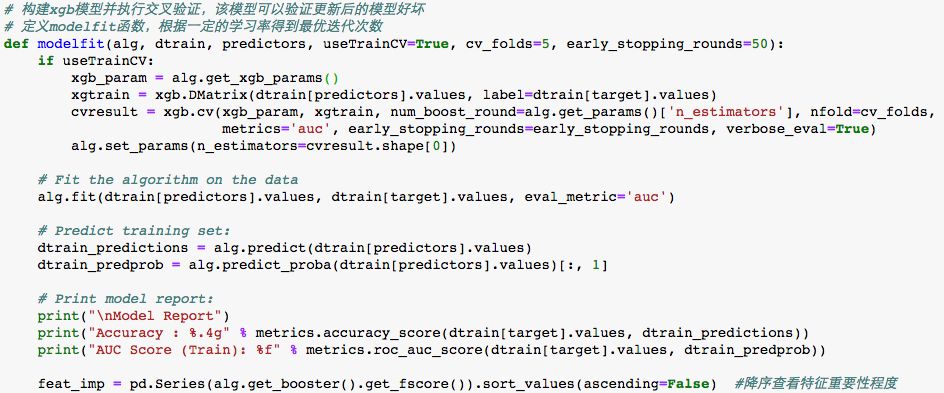
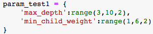
Steps 3, 4, and 5 follow the same parameter tuning ideas as Step 2, which will not be elaborated on here. Please refer to the code for understanding.

Step6: Reduce the learning rate and increase the corresponding maximum number of iterations. The parameter tuning idea is consistent with Step 1, obtaining the optimal number of iterations and outputting the cross-validation rate results.

When the number of iterations is 2346, the optimal classification result is obtained (as shown in the figure below).

5. Summary of XGBoost Parameter Tuning

XGBoost is a high-performance learning model algorithm. When you are unsure how to tune the model parameters, you can refer to the steps in the previous section for parameter tuning. This section describes my understanding of XGBoost parameter tuning based on the previous section’s content and my project experience. If there are any errors, please feel free to point them out.

(1) Model Initialization. When initializing model parameters, we try to keep the model’s complexity high, and then gradually reduce the model’s complexity through parameter tuning. For example, in the previous section, the initialized parameters: minimum weight for leaf nodes is 0, maximum tree depth is 5, and minimum loss function decrease value is 0; these parameter initializations all complicate the model.

(2) Learning Rate and Maximum Iteration Count. The tuning of these two parameters must be interconnected. The larger the learning rate, the fewer maximum iterations required to achieve the same performance of the model; conversely, the smaller the learning rate, the more maximum iterations are needed. XGBoost requires multiple iterations for each parameter update, so learning rate and maximum iteration count are the first parameters to consider, and the focus of learning rate and maximum iteration parameters is not to improve the model’s classification accuracy, but to enhance the model’s generalization ability. Therefore, when the model’s classification accuracy is very high, we should reduce the learning rate in the final step to improve the model’s generalization ability.

(3) Gradually Reduce Model Complexity. Parameters like maximum tree depth and minimum leaf node weight are factors affecting model complexity. This depends on personal experience. The parameter tuning order in the fourth section is: maximum tree depth and minimum leaf node weight -> minimum loss function decrease value -> row sampling and column sampling -> regularization parameters. In practical projects, I generally follow this order for tuning parameters; if there are different understandings, I welcome discussions.

(4) Feature Engineering: If the model’s accuracy is very low, I recommend not tuning parameters for now, but rather focusing on features and training data. Features and data determine the model’s upper limit; the model only approaches this limit.

References:

https://www.analyticsvidhya.com/blog/2016/03/complete-guide-parameter-tuning-xgboost-with-codes-python/

https://xgboost.readthedocs.io/en/latest/

I am Dong Ge, and I am currently creating the “100 Cool Operations of Pandas” series topic. Feel free to subscribe. After subscribing, article updates will be pushed to your subscription account in real-time, and you won’t miss any articles.

Finally, I would like to share with you 10 Electronic Books on Data Mining, including data analysis, statistics, data mining, and machine learning.

These are now shared for free. Readers who need them can download and study by replying with the keyword: Data Mining in the public account “Data Mining Engineer“.