Click on the above “Beginner’s Guide to Vision” to select and add “Star” or “Pin“
Heavy content delivered first
Author | OpenMMLab Editor | Jishi Platform
Original link: https://zhuanlan.zhihu.com/p/430123077
Introduction
With the rapid development of deep learning, the explosion of model parameters has raised increasingly high requirements for GPU memory capacity. How to train models on single GPUs with small memory has always been a concern. This article provides a brief analysis of some commonly used memory-saving strategies using the MMCV open-source library.
0 Introduction
The memory-saving strategies in PyTorch discussed in this article include:
-
Mixed Precision Training -
Large Batch Training, also known as Gradient Accumulation -
Gradient Checkpointing
1 Mixed Precision Training
Mixed Precision Training, also known as Automatic Mixed Precision (AMP), is commonly referred to as FP16. The principles, source code implementation, and usage of AMP in MMCV have been detailed in previous articles, with specific links provided:
OpenMMLab: Detailed Explanation of torch.cuda.amp: Automatic Mixed Precision
https://zhuanlan.zhihu.com/p/348554267
OpenMMLab: The Correct Way to Use Mixed Precision Training AMP in OpenMMLab
https://zhuanlan.zhihu.com/p/375224982
As the previous two articles have analyzed in detail, this article will only briefly describe the principles and specific usage.
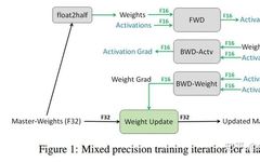
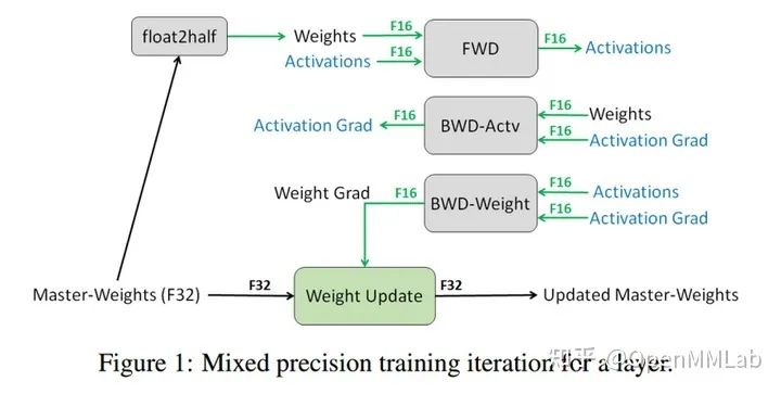
Considering that the gradient magnitudes during training are mostly very small, the default training format is FP32. If we can train directly in FP16 format, it theoretically reduces memory usage by half, allowing for faster training and larger batch sizes. However, training directly in FP16 can lead to overflow issues, resulting in NaNs or failed parameter updates. The emergence of AMP is to solve this problem, and its core idea is mixed precision training + dynamic loss scaling:
-
Maintain a copy of the model with FP32 precision -
In each iteration
-
Copy and convert to FP16 model -
Forward propagation (FP16 model parameters), at this time weights and activations are FP16 -
Loss multiplied by scale factor s -
Backward propagation (FP16 model parameters and parameter gradients), at this time gradients are also FP16 -
Parameter gradients multiplied by 1/s -
Use FP16 gradients to update FP32 model parameters
Using AMP in MMCV can be divided into two cases:
-
Using MMCV’s AMP in upstream libraries like MMDetection -
Users want to simply call AMP in MMCV without relying on upstream libraries
(1) How to Use MMCV’s AMP in OpenMMLab Upstream Libraries
Taking MMDetection as an example, the usage is very simple; just set it in the configuration:
fp16 = dict(loss_scale=512.)  # Static scale

# Dynamic scale
fp16 = dict(loss_scale='dynamic')

# Flexibly enable dynamic scale through dictionary
fp16 = dict(loss_scale=dict(init_scale=512.,mode='dynamic'))
These three different settings have similar performance on most models. If you do not want to set loss_scale, you can simply use loss_scale='dynamic'.
(2) Calling AMP in MMCV
Directly calling AMP in MMCV usually means that users may have AMP functionality supported in other libraries or their own codebases. It is important to emphasize that PyTorch officially began supporting AMP only in version 1.6 and later. Meanwhile, MMCV’s AMP support starts from version 1.3 and later. If you want to use AMP in versions 1.3 or 1.5, using MMCV is a very good choice.
Using MMCV’s AMP functionality requires following these steps:
-
Apply the auto_fp16 decorator to the model’s forward function -
Set the model’s fp16_enabled to True to enable AMP training; otherwise, it will not take effect -
If AMP is enabled, the corresponding FP16 optimizer configuration Fp16OptimizerHook must also be set -
At different training moments, call Fp16OptimizerHook. If you are using MMCV’s Runner module, you can directly input the parameters from step 3 into the Runner -
(Optional) If you want certain operations to run in FP32, you can introduce the force_fp32 decorator at the appropriate places
# 1 Apply to the forward function
class ExampleModule(nn.Module):

    @auto_fp16()
    def forward(self, x, y):
        return x, y

# 2 If AMP is enabled, add the enabling flag
model.fp16_enabled = True

# 3 Configure Fp16OptimizerHook
optimizer_config = Fp16OptimizerHook(
    **cfg.optimizer_config, **fp16_cfg, distributed=distributed)

# 4 Pass to runner
runner.register_training_hooks(cfg.lr_config, optimizer_config,
                               cfg.checkpoint_config, cfg.log_config,
                               cfg.get('momentum_config', None))

# 5 Optional
class ExampleModule(nn.Module):

    @auto_fp16()
    def forward(self, x, y):
        features=self._forward(x, y)
        loss=self._loss(features,labels)
        return loss

    def _forward(self, x, y):
       pass

    @force_fp32(apply_to=('features',))
    def _loss(features,labels) :
        pass
Note that force_fp32 needs to be effective; fp16_enabled must still be True for it to take effect.
2 Large Batch Training (Gradient Accumulation)
Large Batch Training is commonly referred to as the gradient accumulation strategy. Typically, the training process in PyTorch for one iteration is:
y_pred = model(xx)
loss = loss_fn(y_pred, y)
loss.backward()
optimizer.step()
optimizer.zero_grad()
Whereas under the gradient accumulation strategy, a typical training process for one iteration is:
y_pred = model(xx)
loss = loss_fn(y_pred, y)

loss = loss / cumulative_iters
loss.backward()

if current_iter % cumulative_iters==0:
    optimizer.step()
    optimizer.zero_grad()
The core idea is to accumulate gradients from the previous iterations and then perform a unified parameter update, thereby achieving a larger effective batch size. It is important to note that if the model includes layers that consider batch information, such as Batch Normalization, there may be slight performance differences.
For details, refer to:
https://github.com/open-mmlab/mmcv/pull/1221
The gradient accumulation functionality has already been implemented in MMCV, with the core code located in mmcv/runner/hooks/optimizer.py. The GradientCumulativeOptimizerHook is implemented using hooks, similar to AMP. The usage is similar; just replace Fp16OptimizerHook from the first section with GradientCumulativeOptimizerHook or GradientCumulativeFp16OptimizerHook. The core implementation is as follows:
@HOOKS.register_module()
class GradientCumulativeOptimizerHook(OptimizerHook):
    def __init__(self, cumulative_iters=1, **kwargs):

        self.cumulative_iters = cumulative_iters
        self.divisible_iters = 0  # Remaining training iterations divisible by cumulative_iters
        self.remainder_iters = 0  # Remaining accumulation times
        self.initialized = False

    def after_train_iter(self, runner):
        # Only need to run once
        if not self.initialized:
            self._init(runner)

        if runner.iter < self.divisible_iters:
            loss_factor = self.cumulative_iters
        else:
            loss_factor = self.remainder_iters

        loss = runner.outputs['loss']
        loss = loss / loss_factor
        loss.backward()

        if (self.every_n_iters(runner, self.cumulative_iters)
                or self.is_last_iter(runner)):

            runner.optimizer.step()
            runner.optimizer.zero_grad()

    def _init(self, runner):

        residual_iters = runner.max_iters - runner.iter

        self.divisible_iters = (
            residual_iters // self.cumulative_iters * self.cumulative_iters)
        self.remainder_iters = residual_iters - self.divisible_iters

        self.initialized = True
It is important to understand the meanings of divisible_iters and remainder_iters:
(1) Training from Scratch
In this case, when training starts, iter=0, and the total iterations max_iters=102, with a gradient accumulation count of 4. Since 102 cannot be evenly divided by 4, the last 2 iterations (102 – (102 // 4)*4) need to be considered separately. In the last 2 training iterations, loss_factor should not be divided by 4 but by 2 for the most reasonable approach. Here, remainder_iters=2 and divisible_iters=100, residual_iters=102.
(2) Resume Training
If you exit during gradient accumulation and then resume training, iter will not be 0, and since the optimizer object needs to be re-initialized, you need to recalculate residual_iters to ensure that the remaining iterations that cannot be accumulated can be correctly calculated.
3 Gradient Checkpointing
Gradient checkpointing is a method to trade training time for GPU memory. Its core principle is to recompute the intermediate activation values of the neural network during backpropagation instead of storing them during forward propagation. The corresponding functionality has been implemented in the torch.utils.checkpoint package. The brief implementation process is: the forward function passed to the checkpoint during the forward phase runs in _torch.no_grad_ mode, saving only the input parameters and the forward function, and recomputing its forward output values during the backward phase.
The specific usage is very simple; for example, in ResNet’s BasicBlock:
def forward(self, x):
    def _inner_forward(x):
        identity = x
        out = self.conv1(x)
        out = self.norm1(out)
        out = self.relu(out)
        out = self.conv2(out)
        out = self.norm2(out)
        if self.downsample is not None:
            identity = self.downsample(x)
        out += identity
        return out

    # The x.requires_grad check is very necessary
    if self.with_cp and x.requires_grad:
        out = cp.checkpoint(_inner_forward, x)
    else:
        out = _inner_forward(x)
    out = self.relu(out)
    return out
self.with_cp being True indicates that the gradient checkpointing functionality should be enabled.
When using checkpoint, it is important to note the following points:
-
The first layer of the model cannot use checkpoint, or all inputs in the forward must not have their requires_grad attribute set to False, because the internal implementation relies on the requires_grad attribute of the inputs to determine whether the output needs gradients. Typically, the first layer’s input is an image tensor, which usually has requires_grad set to False. If you use checkpoint on the first layer, it means that this forward function will have no gradients, meaning there will be no parameter updates, which is unnecessary. For more details, refer to https://discuss.pytorch.org/t/use-of-torch-utils-checkpoint-checkpoint-causes-simple-model-to-diverge/116271. If you apply checkpoint to the first layer, PyTorch will print a warning None of the inputs have requires_grad=True. Gradients will be Non. -
For layers with randomness in forward, such as dropout, ensure that preserve_rng_state is set to True (which is the default, so no need to worry). Once the flag is set to True, it stores the RNG state during forward and reads the RNG during backpropagation to ensure consistency in outputs between two forward passes. If you are certain that you do not need to save the RNG, you can set preserve_rng_state to False to skip unnecessary logic. -
For other considerations, refer to the official documentation https://pytorch.org/docs/stable/checkpoint.html#.
The core implementation is as follows:
class CheckpointFunction(torch.autograd.Function):

    @staticmethod
    def forward(ctx, run_function, preserve_rng_state, *args):
        # Check if input parameters require gradients
        check_backward_validity(args)
        # Save necessary states
        ctx.run_function = run_function
        ctx.save_for_backward(*args)
        with torch.no_grad():
            # Run once in no_grad model
            outputs = run_function(*args)
        return outputs

    @staticmethod
    def backward(ctx, *args):
        # Read input parameters
        inputs = ctx.saved_tensors
        # Stash the surrounding rng state, and mimic the state that was
        # present at this time during forward. Restore the surrounding state
        # when we're done.
        rng_devices = []
        with torch.random.fork_rng(devices=rng_devices, enabled=ctx.preserve_rng_state):
            # Detach the current nodes that do not need consideration
            detached_inputs = detach_variable(inputs)
            # Run again
            with torch.enable_grad():
                outputs = ctx.run_function(*detached_inputs)

        if isinstance(outputs, torch.Tensor):
            outputs = (outputs,)
        # Compute gradients for this subgraph
        torch.autograd.backward(outputs, args)
        grads = tuple(inp.grad if isinstance(inp, torch.Tensor) else inp
                      for inp in detached_inputs)
        return (None, None) + grads
4 Experimental Validation
To validate whether the above strategies can indeed save memory, the mmdetection library was used for verification, with the basic environment as follows:
GPU: GeForce GTX 1660
PyTorch: 1.7.1
CUDA Runtime: 10.1
MMCV: 1.3.16
MMDetection: 2.17.0
(1) Base
-
Dataset: PASCAL VOC -
Algorithm: RetinaNet, corresponding configuration file: retinanet_r50_fpn_1x_voc0712.py -
To prevent the learning rate from being too high and causing NaNs during training, set the learning rate to 0.01/8=0.00125 -
Batch size set to 2
(2) Mixed Precision AMP
Simply add the following configuration on top of the base configuration:
fp16 = dict(loss_scale=512.)
(3) Gradient Accumulation
Replace optimizer_config in the base configuration with the following:
# Accumulate 2 times
optimizer_config = dict(type='GradientCumulativeOptimizerHook', cumulative_iters=2)
(4) Gradient Checkpointing
Enable the with_cp flag in the backbone section on top of the base configuration:
model = dict(backbone=dict(with_cp=True),
             bbox_head=dict(num_classes=20))
Each experiment iterated a total of 1300 times, recording memory usage and total training time.
| Configuration | Memory Usage (MB) | Training Duration |
|---|---|---|
| Base | 2900 | 7 minutes 45 seconds |
| Mixed Precision AMP | 2243 | 36 minutes |
| Gradient Accumulation | 3177 | 7 minutes 32 seconds |
| Gradient Checkpointing | 2590 | 8 minutes 37 seconds |
-
Comparing base and AMP, since the experimental GPU does not support AMP, it can only save memory, and the speed will be particularly slow. If the GPU itself supports AMP, it can achieve both memory savings and speedup. -
Comparing base and gradient accumulation, it can be seen that with the same batch size, accumulating gradients 2 times is equivalent to doubling the batch size, but the memory increase is minimal. If the batch size is halved, it can save about half the memory under the same batch size. -
Comparing base and gradient checkpointing, it can be seen that it can save some memory, but training time will increase slightly.
From the above simple experiments, it can be concluded that AMP, gradient accumulation, and gradient checkpointing can indeed reduce memory usage to varying degrees, and these three strategies are orthogonal and can be used simultaneously.
5 Conclusion
This article briefly describes three memory-saving strategies integrated into MMCV that can be enabled with a single configuration line. These strategies are commonly used and well-established. As model sizes continue to grow, many new strategies have emerged, such as model parameter compression, dynamic memory optimization, using CPU memory as a temporary storage strategy, and the latest support for ZeroRedundancyOptimizer in PyTorch 1.10 under distributed conditions.
Quick links to the MMCV algorithm library, welcome everyone to star:
https://github.com/open-mmlab/mmcv
Download 1: Chinese Tutorial on OpenCV-Contrib Extension Modules

Reply "Chinese Tutorial on Extension Modules" in the backend of the "Beginner's Guide to Vision" public account to download the first complete Chinese tutorial on OpenCV extension modules, covering installation of extension modules, SFM algorithms, stereo vision, object tracking, biological vision, super-resolution processing, and over twenty chapters of content.

Download 2: 52 Lectures on Practical Python Vision Projects

Reply "Practical Python Vision Projects" in the backend of the "Beginner's Guide to Vision" public account to download 31 practical vision projects including image segmentation, mask detection, lane line detection, vehicle counting, eyeliner addition, license plate recognition, character recognition, emotion detection, text content extraction, facial recognition, etc., to help quickly learn computer vision.

Download 3: 20 Lectures on Practical OpenCV Projects

Reply "20 Practical OpenCV Projects" in the backend of the "Beginner's Guide to Vision" public account to download 20 practical projects based on OpenCV, achieving advanced learning in OpenCV.

Group Chat

Welcome to join the reader group of the public account to communicate with peers. Currently, there are WeChat groups for SLAM, 3D vision, sensors, autonomous driving, computational photography, detection, segmentation, recognition, medical imaging, GANs, algorithm competitions, etc. (will gradually be subdivided in the future). Please scan the WeChat ID below to join the group, and note: "Nickname + School/Company + Research Direction", for example: "Zhang San + Shanghai Jiao Tong University + Vision SLAM". Please follow the format; otherwise, you will not be approved. After successfully adding, you will be invited to relevant WeChat groups based on research direction. Please do not send advertisements in the group; otherwise, you will be removed. Thank you for your understanding~