

RNN is a popular model for processing time series data, demonstrating significant effectiveness in fields such as NLP and time series forecasting.As this article focuses on the practical application of RNN rather than theoretical knowledge, interested readers are encouraged to study RNN systematically.
The following example is implemented using TensorFlow.Using TensorFlow to implement RNN or LSTM is quite convenient; you just need to create RNN or LSTM neurons and then build the network. However, RNN or LSTM differs from conventional neural networks because it processes time series data, which imposes different requirements on data formatting during batch training.
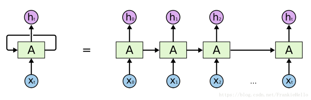
Here is a common RNN model:
Data Preprocessing
First, we need to import the necessary libraries and split the data into training and testing sets.Additionally, we need to normalize the data:
import pandas as pd
import numpy as np
import tensorflow as tf
import matplotlib.pyplot as plt
from sklearn.cluster import k_means
from sklearn.preprocessing import MinMaxScaler

df = pd.read_csv('SP_2000_2017_Daily.csv')
data = df[:4100].Close.as_matrix().astype(float)
data = np.reshape(data, (-1, 1))
mm = MinMaxScaler(feature_range=(-1,1))
data = mm.fit_transform(data)
print(data.shape)
x, y = set_window(data)
# --------------------------Split training and testing datasets--------------------
train_x = x[:2000]
train_y = y[:2000]
test_x = x[2000:4000]
test_y = y[2000:4000]
Since the structure of RNN requires input in windows, we also need to segment the data into windows:
def set_window(data, windowSize = WINDOW_SIZE):
    x = []
    label = []
    length = len(data)
    for i in range(length - windowSize):
        x.append(data[i:i+windowSize, 0])
        label.append(data[i+windowSize])
    return x, label
Network Construction
Once the data is prepared, we need to build the network.
The accepted training data has a shape of [batchSize, 4], which means using the first 4 data points to predict the next one.
hidden_size refers to the number of neurons in an LSTM or RNN unit, represented as a box A in the structure diagram, which can be imagined to contain that many neurons.
class RNN(object):
    def __init__(self):
        self.stateNum = WINDOW_SIZE
        self.batchSize = 50
        self.time_step = 20  # Time step
        self.hidden_size = 100  # Number of hidden units
        self._build_net()
        self.sess = tf.Session()
        self.sess.run(tf.global_variables_initializer())

    def _build_net(self):
        self.x = tf.placeholder(tf.float32, [None, self.stateNum])
        self.y = tf.placeholder(tf.float32, [None, 1])

        w = tf.Variable(tf.truncated_normal([self.hidden_size, 1], stddev=0.1))
        b = tf.Variable(tf.constant(0.1, shape=[1]))

        input_data = tf.reshape(self.x, [-1, self.stateNum, 1])
        rnn_cell = tf.nn.rnn_cell.BasicRNNCell(self.hidden_size)

        batchSize = tf.shape(self.x)[0]
        init_state = rnn_cell.zero_state(batchSize, tf.float32)
        outputs_rnn, final_state = tf.nn.dynamic_rnn(rnn_cell, input_data, dtype=tf.float32, initial_state=init_state)
        output = tf.reshape(outputs_rnn, [-1, self.hidden_size])
        self.prediction = tf.matmul(final_state, w) + b
        self.loss = tf.reduce_mean(tf.square(self.y - self.prediction))
        self.train = tf.train.AdamOptimizer(0.001).minimize(self.loss)

    def train_net(self, x, label):
        batch_num = len(x) // self.batchSize
        for epoch in range(100):
            loss_sum = 0
            for i in range(batch_num):
                dict = {self.x: x[i * self.batchSize:(i + 1) * self.batchSize],
                         self.y: label[i * self.batchSize:(i + 1) * self.batchSize]}
                loss, _, pre = self.sess.run([self.loss, self.train, self.prediction], feed_dict=dict)
                loss_sum += loss
            print(str(epoch) + str(':') + str(loss_sum))

    def predict(self, x):
        dict = {self.x: x}
        prediction = self.sess.run(self.prediction, feed_dict=dict)
        return prediction
The key point in the above code is why we reshape into this structure.
First, the reshaped structure is passed as a parameter to tf.nn.dynamic_rnn; let’s first look at the parameter introduction of this function:
    cell: An instance of RNNCell.
    inputs: The RNN inputs.  If `time_major == False` (default), this must be a `Tensor` of shape:
        `[batch_size, max_time, ...]`, or a nested tuple of such elements.  If `time_major == True`, this must be a `Tensor` of shape:
        `[max_time, batch_size, ...]`, or a nested tuple of such elements.  This may also be a (possibly nested) tuple of Tensors satisfying this property.  The first two dimensions must match across all the inputs, but otherwise the ranks and other shape components may differ.  In this case, input to `cell` at each time-step will replicate the structure of these tuples, except for the time dimension (from which the time is taken).
    sequence_length: (optional) An int32/int64 vector sized `[batch_size]`.  Used to copy-through state and zero-out outputs when past a batch element's sequence length.  So it's more for correctness than performance.
    initial_state: (optional) An initial state for the RNN.  If `cell.state_size` is an integer, this must be a `Tensor` of appropriate type and shape `[batch_size, cell.state_size]`.  If `cell.state_size` is a tuple, this should be a tuple of tensors having shapes `[batch_size, s] for s in cell.state_size`.
    dtype: (optional) The data type for the initial state and expected output.  Required if initial_state is not provided or RNN state has a heterogeneous dtype.
    parallel_iterations: (Default: 32).  The number of iterations to run in parallel.  Those operations which do not have any temporal dependency and can be run in parallel will be.  This parameter trades off time for space.  Values >> 1 use more memory but take less time, while smaller values use less memory but computations take longer.
    swap_memory: Transparently swap the tensors produced in forward inference but needed for back prop from GPU to CPU.  This allows training RNNs which would typically not fit on a single GPU, with very minimal (or no) performance penalty.
    time_major: The shape format of the `inputs` and `outputs` Tensors.  If true, these `Tensors` must be shaped `[max_time, batch_size, depth]`.  If false, these `Tensors` must be shaped `[batch_size, max_time, depth]`.  Using `time_major = True` is a bit more efficient because it avoids transposes at the beginning and end of the RNN calculation.  However, most TensorFlow data is batch-major, so by default this function accepts input and emits output in batch-major form.
    scope: VariableScope for the created subgraph; defaults to "rnn".
The parameter introduction is a bit lengthy; let’s first look at the introduction of inputs, which states that the format of inputs is [batch_size, max_time, …]. Here, max_time refers to the length of the RNN network when unfolded, as shown by t in the diagram.Then the ….. indicates the dimension of the input x.This explains why reshaping to [-1, 4, 1] is reasonable -1 indicates that we don’t care about that dimension; if our batch_size is 50, -1 will be computed as 50*4/4/1=50, meaning 50 batches are input to the RNN network, each with a length of 4, where each box accepts 1-dimensional data.
There are two outputs: one is outputs and the other is state.
The outputs are shaped as [batch_size, max_time, cell.out_size].For the network we designed, this corresponds to a shape of [50, 4, 100], meaning that this batch contains the outputs of 50 groups of input data processed through 4 units, each with 100 neurons.In comparison with conventional NN, the output of a normal NN should be similar to [50, 100], but RNN yields a result of [50, 4, 100] after unfolding.
Once we understand outputs, understanding state becomes easier.This state is the final state, which corresponds to the output of the neurons of the last unit after a group of data is input, resulting in an output shape of [50, 100] since we have set 100 neurons.In the RNN model diagram, this corresponds to the output result of the hidden layer of the last box A.
Model Training
The model training part is quite simple: instantiate the RNN object and call its methods to train on the training set, then test on the testing set:
rnn = RNN()
rnn.train_net(train_x, train_y)
result = rnn.predict(test_x)
prediction = mm.inverse_transform(result)
y = mm.inverse_transform(test_y)
print(result)
print(prediction)
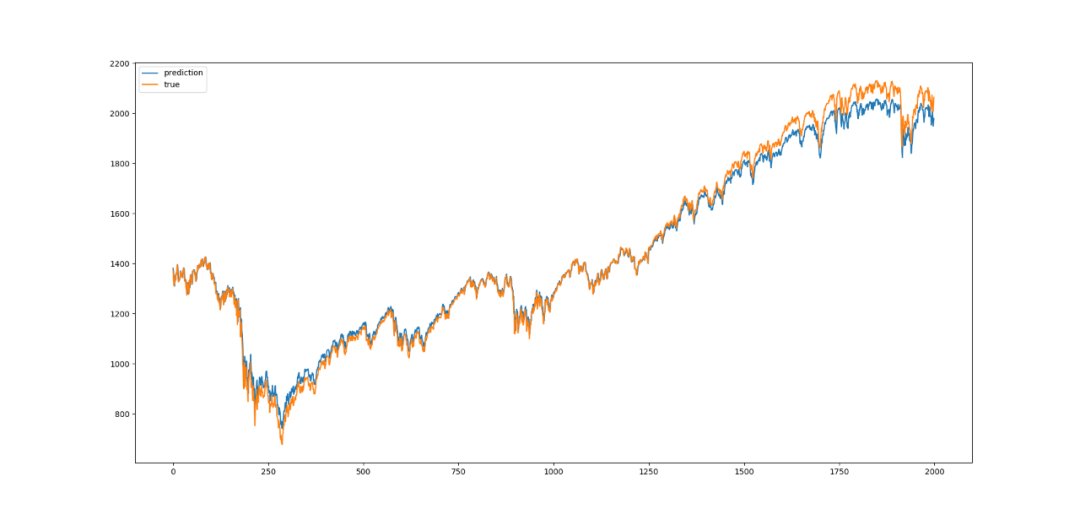
fig = plt.figure()
ax = fig.add_subplot(111)
ax.plot(range(len(prediction)), prediction)
ax.plot(range(len(y)), y)
ax.legend(['prediction', 'true'])
cal_accr(prediction, y)
plt.show()Training Results
Since the neuron count and window size were not tuned, the prediction results are not very satisfactory. Interested readers can try their own data and adjust the parameters:
Conclusion
(Editor’s Note)
Finally, regarding how to learn the mathematical foundations of machine learning, I recommend a column by a friend from Tsinghua on GitChat, which provides an accessible explanation of mathematical probability and statistics in machine learning. It’s worth studying for those without a background in math and statistics (29 yuan, about the price of a meal).