
Author: Chen Yang
Editor: Huang Junjia
Introduction
Hi everyone, I am the pirate captain from Ocean University of China. Today, I am starting a new series. During this time, I have been helping Xuan Jie run experimental codes and conducted many comparative experiments. I found that the implementation of Keras is very good in terms of code readability, and building neural networks is as fun as playing with Lego blocks. 😯. Not just demos, I will also teach you how to build real models like Alexnet, Vggnet, Resnet, etc. in a series of Keras tutorials, and how to run them on GPU servers.
01
Introduction to Keras
Keras is a high-level neural network API written in Python that can run on top of TensorFlow, CNTK, or Theano. The focus of Keras development is to support fast experimentation. The ability to turn your ideas into experimental results with minimal delay is key to good research.
If you need a deep learning library in the following scenarios, please use Keras:
Allows for simple and quick prototyping (due to its user-friendly, highly modular, and extensible nature).
Simultaneously supports convolutional neural networks and recurrent neural networks, as well as combinations of both.
Runs seamlessly on both CPU and GPU.
02
Installation
pip install TensorFlow
pip install keras
03
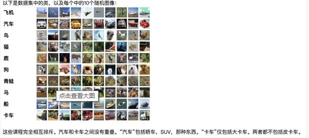
Dataset
This time, we introduce the most common dataset in the lab, CIFAR-10. The computational load of this dataset is about 10 times that of MNIST, and it can barely run on a regular PC, usually we use GPU acceleration on the lab’s server when using this dataset.
Download: https://www.cs.toronto.edu/~kriz/cifar.html
The CIFAR-10 dataset consists of 60,000 32×32 color images in 10 classes, with 6,000 images per class. It has 50,000 training images and 10,000 testing images.
The dataset is divided into five training batches and one testing batch, with each batch containing 10,000 images. The testing batch contains 1,000 randomly selected images from each category. The training batches contain the remaining images in random order, but some training batches may contain more images from one category than another. In total, the training batches contain 5,000 images from each category.
Here, we can take advantage of Keras’s inherent strengths to easily load the dataset.
import keras
from keras.datasets import cifar10
(ps, here we have a command to run in the terminal)
sudo apt-get install graphviz
pip install pydot
04
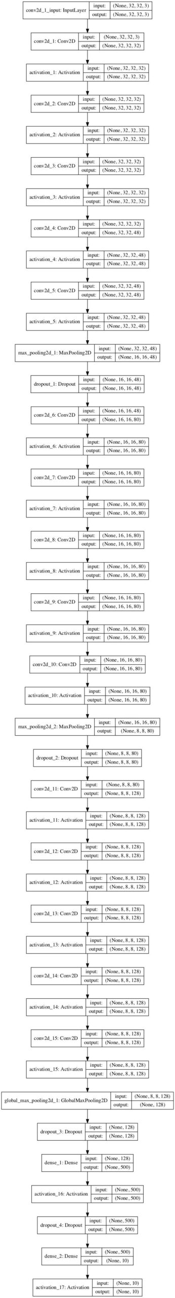
CNN Network Structure Model
Emmmm, the network structure is quite deep.
05
Header Files
#coding=utf-8
import keras
from keras.datasets import cifar10
from keras.preprocessing.image import ImageDataGenerator
from keras.models import Sequential
from keras.layers import Dense, Dropout, Flatten
from keras.layers import Conv2D, MaxPooling2D, ZeroPadding2D, GlobalMaxPooling2D
Sequential: Sequential model
Dense: Fully connected, abbreviated as FC
Flatten: The process from s4 to c5 in the above image, equivalent to flattening the 16*5*5 feature map into a 400-dimensional feature vector, and then compressing it into a 120-dimensional feature vector through full connection.
Conv2D: 2D convolution
ImageDataGenerator: Image augmentation, a built-in data augmentation function in Keras that can make our dataset larger and improve the generalization ability of the trained network.
Dropout: Dropout layer, neurons are deactivated with a certain probability, which can prevent overfitting.
Activation: Activation layer, activates the tensor through the activation function.
MaxPooling2D: 2D down-sampling, referred to as subsampling in the article.
to_categorical: Converts a 1D vector into a num_class-dimensional one-hot encoding.
from keras.datasets import cifar10: Keras comes with the CIFAR-10 dataset.
plot_model: Prints the model we will build, equivalent to visualizing the model.
06
Loading the Dataset
batch_size = 32
num_classes = 10
epochs = 1600
data_augmentation = True

# The data, shuffled and split between train and test sets:
(x_train, y_train), (x_test, y_test) = cifar10.load_data()
print('x_train shape:', x_train.shape)
print(x_train.shape[0], 'train samples')
print(x_test.shape[0], 'test samples')
x_train = x_train.astype('float32')
x_test = x_test.astype('float32')
x_train /= 255
x_test /= 255

# Convert class vectors to binary class matrices.
y_train = keras.utils.to_categorical(y_train, num_classes)
y_test = keras.utils.to_categorical(y_test, num_classes)
X_train, y_train: Training sample data and labels
X_test, y_test: Testing sample data and labels
50,000 train samples
10,000 test samples
x_train’s shape=
(50000,32,32,3), dtype=int, 0~255
y_train’s shape= (50000, 10)
07
Building the Network
model = Sequential()

model.add(Conv2D(32, (3, 3), padding='same',
                 input_shape=x_train.shape[1:]))
model.add(Activation('relu'))
model.add(Conv2D(32, (3, 3), padding='same',
                 input_shape=x_train.shape[1:]))
model.add(Activation('relu'))
model.add(Conv2D(32, (3, 3), padding='same',
                 input_shape=x_train.shape[1:]))
model.add(Activation('relu'))
model.add(Conv2D(48, (3, 3), padding='same',
                 input_shape=x_train.shape[1:]))
model.add(Activation('relu'))
model.add(Conv2D(48, (3, 3), padding='same',
                 input_shape=x_train.shape[1:]))
model.add(Activation('relu'))
model.add(MaxPooling2D(pool_size=(2, 2)))
model.add(Dropout(0.25))

model.add(Conv2D(80, (3, 3), padding='same',
                 input_shape=x_train.shape[1:]))
model.add(Activation('relu'))
model.add(Conv2D(80, (3, 3), padding='same',
                 input_shape=x_train.shape[1:]))
model.add(Activation('relu'))
model.add(Conv2D(80, (3, 3), padding='same',
                 input_shape=x_train.shape[1:]))
model.add(Activation('relu'))
model.add(Conv2D(80, (3, 3), padding='same',
                 input_shape=x_train.shape[1:]))
model.add(Activation('relu'))
model.add(Conv2D(80, (3, 3), padding='same',
                 input_shape=x_train.shape[1:]))
model.add(Activation('relu'))
model.add(MaxPooling2D(pool_size=(2, 2)))
model.add(Dropout(0.25))

model.add(Conv2D(128, (3, 3), padding='same',
                 input_shape=x_train.shape[1:]))
model.add(Activation('relu'))
model.add(Conv2D(128, (3, 3), padding='same',
                 input_shape=x_train.shape[1:]))
model.add(Activation('relu'))
model.add(Conv2D(128, (3, 3), padding='same',
                 input_shape=x_train.shape[1:]))
model.add(Activation('relu'))
model.add(Conv2D(128, (3, 3), padding='same',
                 input_shape=x_train.shape[1:]))
model.add(Activation('relu'))
model.add(Conv2D(128, (3, 3), padding='same',
                 input_shape=x_train.shape[1:]))
model.add(Activation('relu'))
model.add(GlobalMaxPooling2D())
model.add(Dropout(0.25))

model.add(Dense(500))
model.add(Activation('relu'))
model.add(Dropout(0.25))
model.add(Dense(num_classes))
model.add(Activation('softmax'))
model.summary ()
The first and second layers: 32 convolutional kernels of (3*3), with a stride of 1 (default is also 1),
The first network layer must have an input_shape parameter that tells the neural network the size of the input tensor. I recommend writing it as X_train.shape[1:], so that when I change the dataset, I don’t have to change the parameters, and the network will adapt automatically.
data_format=’channels_last’ means telling Keras whether your channel is at the front or back. The default for TensorFlow backend is last, and for Theano backend is first. We are using the default value (do not change it lightly, as it greatly affects training time; it should conform to the order of the backend, for example, TensorFlow backend does not need to input channels_first; if it is, the actual training will still convert to last, greatly reducing speed).
padding=’same’ (default is valid) means that the feature map size will not change; ‘same’ means padding around to keep the feature map size unchanged.
activation=’relu’ indicates that the activation function is ReLU, which runs after the convolution operation. By default, it is not set.
kernel_initializer=’uniform’ indicates that the convolutional kernel is of the default type.
The third layer: Maxpooling, with fewer parameters, just the size of the pooling kernel, 2*2, with the default stride equal to the size of the pooling.
The 12th layer Dropout
Keras.layers.Dropout(rate, noise_shape=None, seed=None)
Applies Dropout to the input.
Dropout includes setting a proportion of input units to 0 randomly during each update in training, which helps prevent overfitting.
The 16th layer: GlobalMaxPooling2D
Keras.layers.GlobalMaxPooling2D(data_format=None)
Global max pooling for spatial data.
The output size is a 2D tensor of (batch_size, channels).
The last layer: Dense(10) means compressing it to the same dimension as our labels, 10, activated by softmax (softmax is used for multi-class classification).
model.summary(): Prints the network structure and its internal parameters.
08
Network Structure Parameters
_________________________________________________________________
Layer (type)                 Output Shape              Param #
=================================================================
conv2d_1 (Conv2D)            (None, 32, 32, 32)        896
_________________________________________________________________
activation_1 (Activation)    (None, 32, 32, 32)        0
_________________________________________________________________
conv2d_2 (Conv2D)            (None, 32, 32, 32)        9248
_________________________________________________________________
activation_2 (Activation)    (None, 32, 32, 32)        0
_________________________________________________________________
conv2d_3 (Conv2D)            (None, 32, 32, 32)        9248
_________________________________________________________________
activation_3 (Activation)    (None, 32, 32, 32)        0
_________________________________________________________________
conv2d_4 (Conv2D)            (None, 32, 32, 48)        13872
_________________________________________________________________
activation_4 (Activation)    (None, 32, 32, 48)        0
_________________________________________________________________
conv2d_5 (Conv2D)            (None, 32, 32, 48)        20784
_________________________________________________________________
activation_5 (Activation)    (None, 32, 32, 48)        0
_________________________________________________________________
max_pooling2d_1 (MaxPooling2 (None, 16, 16, 48)        0
_________________________________________________________________
dropout_1 (Dropout)          (None, 16, 16, 48)        0
_________________________________________________________________
conv2d_6 (Conv2D)            (None, 16, 16, 80)        34640
_________________________________________________________________
activation_6 (Activation)    (None, 16, 16, 80)        0
_________________________________________________________________
conv2d_7 (Conv2D)            (None, 16, 16, 80)        57680
_________________________________________________________________
activation_7 (Activation)    (None, 16, 16, 80)        0
_________________________________________________________________
conv2d_8 (Conv2D)            (None, 16, 16, 80)        57680
_________________________________________________________________
activation_8 (Activation)    (None, 16, 16, 80)        0
_________________________________________________________________
conv2d_9 (Conv2D)            (None, 16, 16, 80)        57680
_________________________________________________________________
activation_9 (Activation)    (None, 16, 16, 80)        0
_________________________________________________________________
conv2d_10 (Conv2D)           (None, 16, 16, 80)        57680
_________________________________________________________________
activation_10 (Activation)   (None, 16, 16, 80)        0
_________________________________________________________________
max_pooling2d_2 (MaxPooling2 (None, 8, 8, 80)          0
_________________________________________________________________
dropout_2 (Dropout)          (None, 8, 8, 80)          0
_________________________________________________________________
conv2d_11 (Conv2D)           (None, 8, 8, 128)         92288
_________________________________________________________________
activation_11 (Activation)   (None, 8, 8, 128)         0
_________________________________________________________________
conv2d_12 (Conv2D)           (None, 8, 8, 128)         147584
_________________________________________________________________
activation_12 (Activation)   (None, 8, 8, 128)         0
_________________________________________________________________
conv2d_13 (Conv2D)           (None, 8, 8, 128)         147584
_________________________________________________________________
activation_13 (Activation)   (None, 8, 8, 128)         0
_________________________________________________________________
conv2d_14 (Conv2D)           (None, 8, 8, 128)         147584
_________________________________________________________________
activation_14 (Activation)   (None, 8, 8, 128)         0
_________________________________________________________________
conv2d_15 (Conv2D)           (None, 8, 8, 128)         147584
_________________________________________________________________
activation_15 (Activation)   (None, 8, 8, 128)         0
_________________________________________________________________
global_max_pooling2d_1 (Glob (None, 128)               0
_________________________________________________________________
dropout_3 (Dropout)          (None, 128)               0
_________________________________________________________________
dense_1 (Dense)              (None, 500)               64500
_________________________________________________________________
activation_16 (Activation)   (None, 500)               0
_________________________________________________________________
dropout_4 (Dropout)          (None, 500)               0
_________________________________________________________________
dense_2 (Dense)              (None, 10)                5010
_________________________________________________________________
activation_17 (Activation)   (None, 10)                0
=================================================================
Total params: 1,071,542
Trainable params: 1,071,542
Non-trainable params: 0
_________________________________________________________________
Estimated memory usage and computational resources
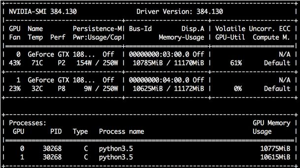
About 10GB of memory, GTX1080TI
09
Compilation and Training
# initiate RMSprop optimizer
opt = keras.optimizers.Adam(lr=0.0001)

# Let's train the model using RMSprop
model.compile(loss='categorical_crossentropy',
              optimizer=opt,
              metrics=['accuracy'])

print("train____________")
model.fit(X_train,y_train,epochs=600,batch_size=128,)
print("test_____________")
loss, acc = model.evaluate(X_test, y_test)
print("loss=", loss)
print("accuracy=", acc)
model.compile: Compiles the model,
optimizer is the optimizer, I chose stochastic gradient descent here, and there are many optimizers available, you can check the official website [here][4]. Here we use Adam, with a learning rate of 0.0001 and momentum decay of 0.
loss=’categorical_crossentropy’: One-hot cross-entropy used for multi-class.
metrics=[‘accuracy’]: Indicates that we want to optimize accuracy.
model.fit(X_train, y_train, epochs=600, batch_size=128,): Trains for 600 epochs with a batch size of 128; by default, regularization is added during training to prevent overfitting.
loss, acc = model.evaluate(X_test, y_test): Tests the samples, by default without using regularization, returning loss and accuracy.
10
Training Method Based on Data Augmentation
if not data_augmentation:
print('Not using data augmentation.')
model.fit(x_train, y_train,
batch_size=batch_size,
epochs=epochs,
validation_data=(x_test, y_test),
shuffle=True, callbacks=[tbCallBack])
else:
print('Using real-time data augmentation.')
# This will do preprocessing and realtime data augmentation:
'''
datagen = ImageDataGenerator(
featurewise_center=False, # set input mean to 0 over the dataset
samplewise_center=False, # set each sample mean to 0
featurewise_std_normalization=False, # divide inputs by std of the dataset
samplewise_std_normalization=False, # divide each input by its std
zca_whitening=False, # apply ZCA whitening
rotation_range=0, # randomly rotate images in the range (degrees, 0 to 180)
width_shift_range=0.1, # randomly shift images horizontally (fraction of total width)
height_shift_range=0.1, # randomly shift images vertically (fraction of total height)
horizontal_flip=True, # randomly flip images
vertical_flip=False) # randomly flip images
'''
datagen = ImageDataGenerator(
featurewise_center=False, # set input mean to 0 over the dataset
samplewise_center=False, # set each sample mean to 0
featurewise_std_normalization=False, # divide inputs by std of the dataset
samplewise_std_normalization=False, # divide each input by its std
zca_whitening=False, # apply ZCA whitening
rotation_range=10, # randomly rotate images in the range (degrees, 0 to 180)
width_shift_range=0.2, # randomly shift images horizontally (fraction of total width)
height_shift_range=0.2, # randomly shift images vertically (fraction of total height)
horizontal_flip=True, # randomly flip images
vertical_flip=False) # randomly flip images
# Compute quantities required for feature-wise normalization
# (std, mean, and principal components if ZCA whitening is applied).
datagen.fit(x_train)
# Fit the model on the batches generated by datagen.flow().
model.fit_generator(datagen.flow(x_train, y_train,
batch_size=batch_size),
steps_per_epoch=x_train.shape[0] // batch_size,
epochs=epochs,
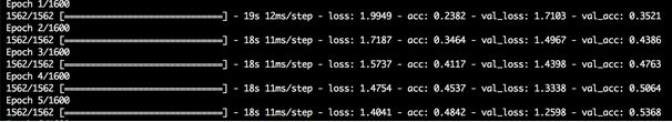
validation_data=(x_test, y_test), callbacks=[tbCallBack])When I run one epoch on my 6-core 12-thread Core i7 MacBook Pro 15, it takes time.
!

Yes… you read that right, overclocked by 543%, still 20 minutes per epoch. Doesn’t it feel like it would take forever to finish 500 epochs?
11
Running on GPU Server
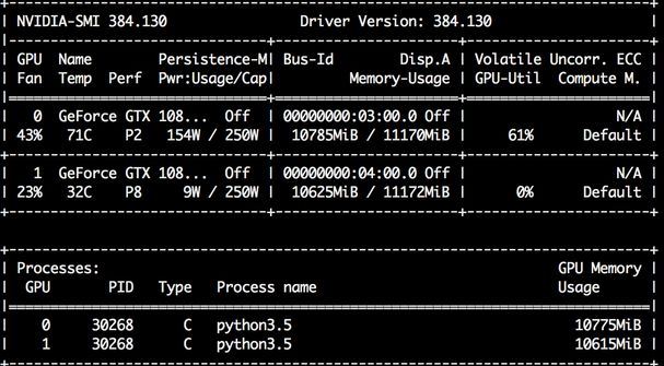
You are not mistaken, this is the power of the GTX1080ti nuclear bomb, a long time later.
12
Model Visualization and Image Saving
import matplotlib.pyplot as plt
import matplotlib.image as mpimg
from keras.utils import plot_model
plot_model(model, to_file='example.png', show_shapes=True)
lena = mpimg.imread('example.png') # Read lena.png in the same directory as the code
# At this point, lena is already a np.array, and you can process it in any way
lena.shape #(512, 512, 3)
plt.imshow(lena) # Display the image
plt.axis('off') # Do not show axes
plt.show()
Traditional model printing code, I think the comments are detailed enough.
13
Model Saving
config = model.get_config()
model = model.from_config(config) 
END
Previous reviews by author Chen Yang
[1] Step-by-step guide to using Keras – building neural networks like Lego (LeNet)
[2] Machine Learning Paper Notes (Seven): A Simple and Effective Network Structure Search
[3] Machine Learning Paper Notes – How to Use Efficient Search Algorithms to Search Network Topologies
[4] The Recent Popular Meta Learning, The Spark Between Genetic Algorithms and Deep Learning
Machine Learning Algorithm Engineer
A dedicated public account

Join the group, learn, and get help
Your attention is our heat,
We will definitely give you the greatest help in learning