Introduction to Mask R-CNN Network

Paper Title: Mask R-CNN
Paper Download Link: https://arxiv.org/abs/1703.06870

Before reading this blog post, you need to understand Faster R-CNN, FPN, and FCN.

Faster R-CNN Video Explanation: https://www.bilibili.com/video/BV1af4y1m7iL?p=3

FPN Video Explanation: https://www.bilibili.com/video/BV1dh411U7D9

FCN Video Explanation: https://www.bilibili.com/video/BV1J3411C7zd

Table of Contents

• 0 Introduction

• 1 Mask R-CNN

• 2 RoI Align

  • 2.1 RoIPool Experiment

  • 2.2 RoIAlign Experiment

• 3 Mask Branch (FCN)

• 4 Other Details

• 4.1 Mask R-CNN Loss

• 4.2 Mask Branch Loss

• 4.3 Mask Branch Prediction Usage

0 Introduction

Mask R-CNN is a paper published in 2017, with the first author being Kaiming He, and indeed, he is that man. Alongside him are the masters of the Faster R-CNN series, Ross Girshick, making it a strong collaboration. The paper also won the Best Paper Award at ICCV 2017 (Marr Prize). After its proposal, this network dominated various tasks on MS COCO, including object detection, instance segmentation, and human keypoint detection tasks. After reading this article, I find the structure of Mask R-CNN to be very simple, flexible, and effective (it merely adds some new branches based on Faster R-CNN as needed).Note that before reading this article, you need to understand Faster R-CNN, FPN, and FCN. If you are not familiar with them, you can refer to the related videos I previously made on Bilibili.

1 Mask R-CNN

The method, called Mask R-CNN, extends Faster R-CNN by adding a branch for predicting an object mask in parallel with the existing branch for bounding box recognition.

Mask R-CNN adds a branch for predicting segmentation masks on the basis of Faster R-CNN (which can predict information about the bounding boxes, class information, and segmentation masks).

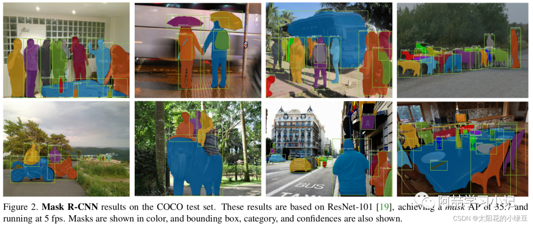
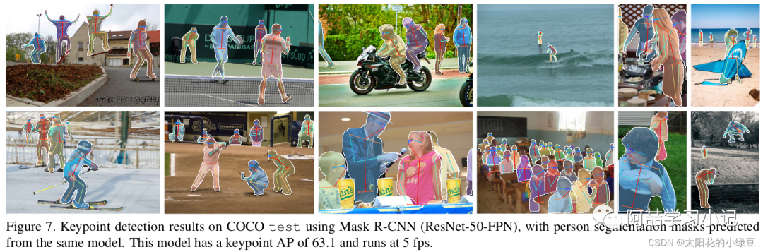
Moreover, Mask R-CNN is easy to generalize to other tasks, e.g., allowing us to estimate human poses in the same framework.

Mask R-CNN can perform both object detection and segmentation simultaneously and can easily be extended to other tasks, such as predicting human keypoints at the same time.

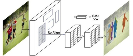
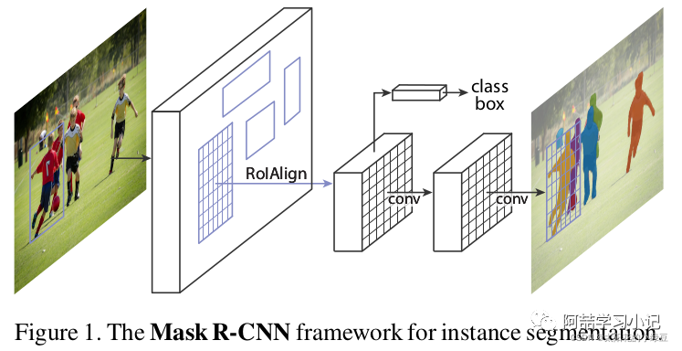
Our method, called Mask R-CNN, extends Faster R-CNN by adding a branch for predicting segmentation masks on each Region of Interest (RoI), in parallel with the existing branch for classification and bounding box regression (Figure 1). The mask branch is a small FCN applied to each RoI, predicting a segmentation mask in a pixel-to-pixel manner.

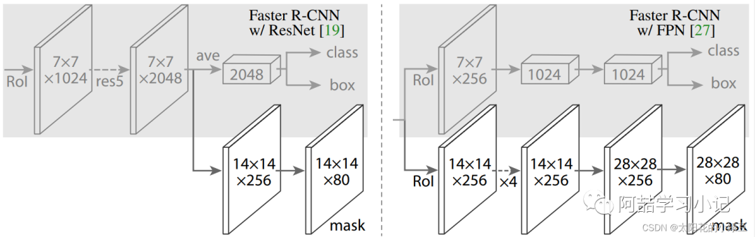
The structure of Mask R-CNN is also very simple; it adds a mask branch (a small FCN) in parallel on top of the RoI obtained through RoIAlign (which was RoIPool in the original Faster R-CNN). As shown in the figure below, Faster R-CNN previously connected a Fast R-CNN detection head on top of the RoI, which is the class, box branch in the figure, and now a mask branch has been added in parallel.

Note that there are slight differences in the Mask branch between Mask R-CNN with and without FPN structure; for Mask R-CNN with FPN structure, the class and box branches do not share the same RoIAlign. During training, for the class, box branch, RoIAlign pools the Proposals obtained from the RPN (Region Proposal Network) to a size of 7x7, while for the Mask branch, RoIAlign pools the Proposals to a size of 14x14. For details, refer to Figure 4 in the original paper.

2 RoI Align

Faster R-CNN was not designed for pixel-to-pixel alignment between network inputs and outputs. This is most evident in how RoIPool, the de facto core operation for attending to instances, performs coarse spatial quantization for feature extraction.

In the previous Faster R-CNN, RoIPool was used to pool the Proposals obtained from the RPN to the same size. This process involves quantization or rounding operations, which can lead to less accurate localization (referred to as the misalignment problem in the paper).

The following diagram illustrates the execution process of RoIPool, which undergoes two rounds of quantization. Assume a Proposal obtained from the RPN has its top-left corner coordinates at (x1, y1) and bottom-right coordinates at (x2, y2), with a stride of 32 for the feature layer relative to the original image. The expected output through RoIPool is a size of 2x2:

• The Proposal is mapped to the feature layer, where the top-left coordinates round to 0 and the bottom-right coordinates round to 4, meaning the top-left coordinates on the feature layer are (0, 0) and the bottom-right coordinates are (4, 4). This corresponds to the area from row 0 to row 4 and column 0 to column 4 on the feature layer (black rectangle). This is the first quantization.
• Since the expected output is 2x2, the mapped Proposal on the feature layer needs to be divided into 2x2 regions. However, the mapped Proposal is 5x5, which cannot be evenly divided, so after forced division, some regions are larger and some are smaller, as shown in the diagram. This is the second quantization.
• Perform maxpool on each sub-region to obtain the output of RoIPool, which corresponds to the Pytorch experiment in section 2.1.

To fix the misalignment, we propose a simple, quantization-free layer, called RoIAlign, that faithfully preserves exact spatial locations.

To address this issue, the authors propose the RoIAlign method to replace RoIPool for obtaining more accurate spatial localization information.

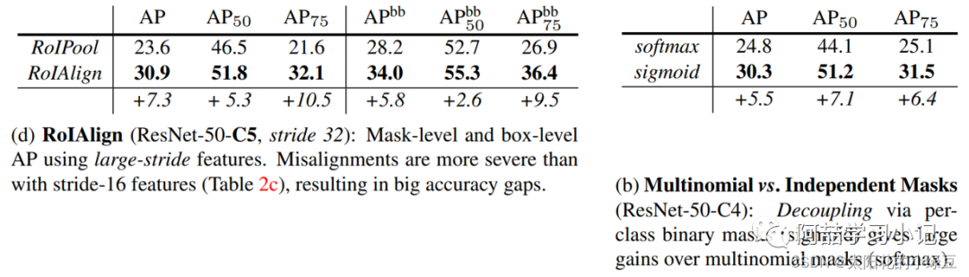
RoIAlign has a large impact: it improves mask accuracy by relative 10% to 50%, showing bigger gains under stricter localization metrics. Second, we found it essential to decouple mask and class prediction: we predict a binary mask for each class independently, without competition among classes, and rely on the network’s RoI classification branch to predict the category.

The authors mention in the paper that replacing RoIPool with RoIAlign improves the accuracy of the segmentation masks by 10% to 50% (see the diagram below d), and decoupling the predicted masks and classes also brought significant improvements (see the diagram below b), which will be discussed in detail later.

The following diagram illustrates the execution process of RoIAlign. Similarly, assume a Proposal obtained from the RPN has its top-left corner coordinates at (x1, y1) and bottom-right coordinates at (x2, y2), with a stride of 32 for the feature layer relative to the original image. The expected output through RoIAlign is a size of 2x2:

• The Proposal is mapped to the feature layer, where the top-left coordinates are (x1, y1) (not rounded), and the bottom-right coordinates are (x2, y2) (not rounded). To facilitate understanding, each element on the feature layer is represented by a point, resulting in the grid shown in the diagram below. The blue rectangle in the diagram represents the Proposal (without quantization).
• Since the expected output is 2x2, the Proposal is divided into 2x2 four sub-regions (without quantization). Next, sampling points are set in each sub-region based on the sampling_ratio; the default value in the original paper is 4, but for convenience, we set the sampling_ratio to 1 here.
• Then, the value of each sampling point in each sub-region is calculated (using bilinear interpolation), and finally, the average of all sampling points in each region is the output for that sub-region.

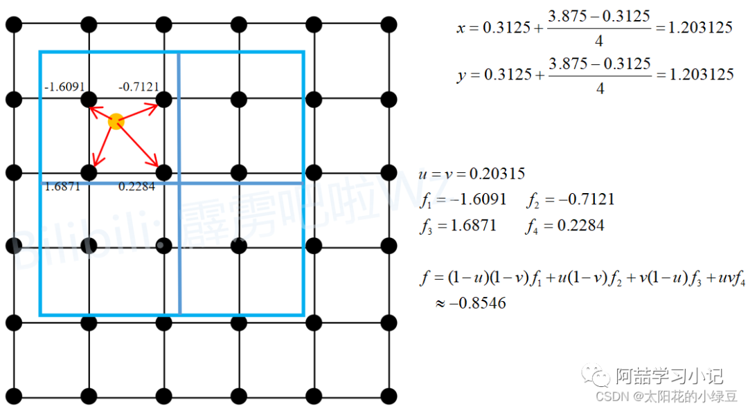
Taking the first sub-region as an example, since we set the sampling_ratio to 1, each sub-region only needs to set one sampling point (the number of sampling points in each sub-region equals the square of the sampling_ratio). The sampling point for the first sub-region is the yellow point in the diagram (the center point of that sub-region), with coordinates (x, y), and then we find the four closest points to that sampling point (indicated by the red arrows in the diagram), and then we can calculate the output corresponding to the sampling point using bilinear interpolation (if you are not familiar with bilinear interpolation, you can refer to the related blog post I wrote earlier). Since there is only one sampling point in this sub-region, the output for this sub-region is (x, y). There is a corresponding Pytorch experiment in section 2.2.

We note that the results are not sensitive to the exact sampling locations, or how many points are sampled, as long as no quantization is performed.

Finally, the authors mention in the paper that the final sampling results are not sensitive to the sampling point locations or the number of sampling points, as long as no quantization is performed.

2.1 RoIPool Experiment

The experiment is conducted in accordance with the previous content for comparison.

The following is the implementation of the RoIPool method in the Torchvision library, and the comparison of the calculated results matches what we just discussed.

import torch
from torchvision.ops import RoIPool

def main():
    torch.manual_seed(1)
    x = torch.randn((1, 1, 6, 6))
    print(f"feature map: \n{x}")
	
	proposal = [torch.as_tensor([[10, 10, 124, 124]], dtype=torch.float32)]
    roi_pool = RoIPool(output_size=2, spatial_scale=1/32)
    roi = roi_pool(x, proposal)
    print(f"roi pool: \n{roi}")


if __name__ == '__main__':
    main()

Terminal Output:

feature map: 

tensor([[[[-1.5256, -0.7502, -0.6540, -1.6095, -0.1002, -0.6092],
          [-0.9798, -1.6091, -0.7121,  0.3037, -0.7773, -0.2515],
          [-0.2223,  1.6871,  0.2284,  0.4676, -0.6970, -1.1608],
          [ 0.6995,  0.1991,  0.1991,  0.0457,  0.1530, -0.4757],
          [-1.8821, -0.7765,  2.0242, -0.0865,  2.3571, -1.0373],
          [ 1.5748, -0.6298,  2.4070,  0.2786,  0.2468,  1.1843]]]])
roi pool: 
tensor([[[[1.6871, 0.4676],
          [2.0242, 2.3571]]]])

2.2 RoIAlign Experiment

The experiment is conducted in accordance with the previous content for comparison.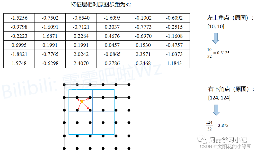

The following is the implementation of the RoIAlign method in the Torchvision library, and the comparison of the calculated results matches what we just discussed.

import torch
from torchvision.ops import RoIAlign


def bilinear(u, v, f1, f2, f3, f4):
    return (1-u)*(1-v)*f1 + u*(1-v)*f2 + (1-u)*v*f3 + u*v*f4


def main():
    torch.manual_seed(1)
    x = torch.randn((1, 1, 6, 6))
    print(f"feature map: \n{x}")
    
    proposal = [torch.as_tensor([[10, 10, 124, 124]], dtype=torch.float32)]
    roi_align = RoIAlign(output_size=2, spatial_scale=1/32, sampling_ratio=1)
    roi = roi_align(x, proposal)
    print(f"roi align: \n{roi}")

    u = 0.203125
    v = 0.203125
    f1 = x[0, 0, 1, 1]  # -1.6091
    f2 = x[0, 0, 1, 2]  # -0.7121
    f3 = x[0, 0, 2, 1]  # 1.6871
    f4 = x[0, 0, 2, 2]  # 0.2284
    print(f"bilinear: {bilinear(u, v, f1, f2, f3, f4):.4f}")


if __name__ == '__main__':
    main()

Terminal Output:

feature map: 

tensor([[[[-1.5256, -0.7502, -0.6540, -1.6095, -0.1002, -0.6092],
          [-0.9798, -1.6091, -0.7121,  0.3037, -0.7773, -0.2515],
          [-0.2223,  1.6871,  0.2284,  0.4676, -0.6970, -1.1608],
          [ 0.6995,  0.1991,  0.1991,  0.0457,  0.1530, -0.4757],
          [-1.8821, -0.7765,  2.0242, -0.0865,  2.3571, -1.0373],
          [ 1.5748, -0.6298,  2.4070,  0.2786,  0.2468,  1.1843]]]])
roi align: 
tensor([[[[-0.8546,  0.3236],
          [ 0.2177,  0.0546]]]])
bilinear: -0.8546

3 Mask Branch (FCN)

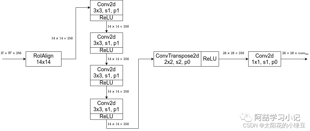
As mentioned earlier, the Mask branches of Mask R-CNN with and without FPN structure are slightly different. The left side of the diagram shows the Mask branch without FPN structure, while the right side shows the Mask branch with FPN structure (the gray part represents the original Faster R-CNN branches predicting box and class information, while the white part represents the Mask branch).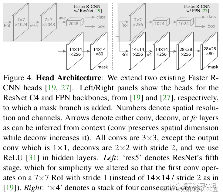Since we generally use networks with FPN in our daily usage, I have also hand-drawn a diagram specifically for the Mask branch with FPN structure:

Previously, when discussing FCN, it was mentioned that FCN predicts a score for each pixel for each category, and then obtains the probability for each category through softmax (there is competition among different categories). The category with the highest probability assigns that pixel to that category. However, in Mask R-CNN, the authors decouple the prediction of masks and classes, meaning that for each input RoI, a mask is predicted for each class independently, without competition among classes. The final corresponding class mask is selected based on the box and class information predicted by the Fast R-CNN branch (there is no competition among different classes). The authors state that this decoupling brought significant improvements. The table below shows the ablation experiment results provided in the original paper, where softmax represents the original FCN method (masks and classes not decoupled), and sigmoid represents the method adopted in Mask R-CNN (masks and classes decoupled).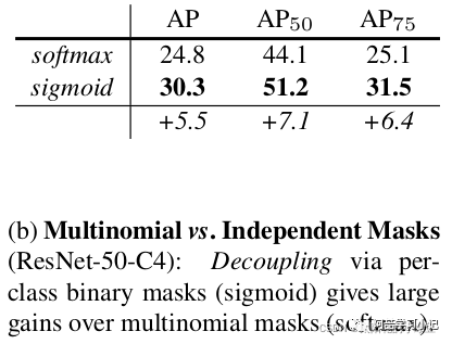

Another detail that needs to be noted is that during training, the targets input to the Mask branch are provided by the RPN, i.e., the Proposals, but during prediction, the targets input to the Mask branch are provided by the Fast R-CNN (i.e., the final predicted targets). Moreover, the Proposals used during training are all positive samples matched in the Fast R-CNN phase. Here I would like to share my personal opinion (which may not be accurate); during training, the Mask branch utilizes the target information provided by the RPN to diversify the training samples (since the bounding boxes provided by the RPN are not very accurate, a target can present different scenarios, similar to random cropping around the target. On the other hand, the outputs obtained through Fast R-CNN are generally quite accurate, and after NMS, the remaining targets are even fewer). During prediction, to obtain more accurate target segmentation information and reduce computational load (the number of targets after Fast R-CNN will be fewer), the target information provided by Fast R-CNN is utilized.

4 Other Details

4.1 Mask R-CNN Loss

The loss of Mask R-CNN is based on Faster R-CNN with the addition of the loss from the Mask branch, which is:

As previously discussed in the video regarding the loss calculation of Faster R-CNN, I will not elaborate on it here. The loss from the Mask branch is the binary cross-entropy loss (Binary Cross Entropy).

4.2 Mask Branch Loss

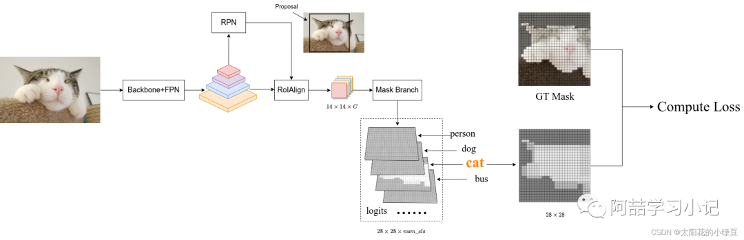
Before discussing the calculation of the Mask branch loss, we need to clarify what logits (the predicted outputs of the network) and targets (the corresponding ground truth) are. As mentioned earlier, during training, the targets input to the Mask branch are the Proposals provided by the RPN, so the predicted logits are the mask information for each category corresponding to each Proposal (note that the predicted mask size is always 28x28). Additionally, the Proposals input here are all positive samples (obtained through sampling in the Fast R-CNN phase), and the corresponding ground truth information (box, class) is also known.

As shown in the figure below, assume a Proposal is obtained (the black rectangle in the figure), and after going through RoIAlign, the corresponding feature information is obtained (shape 14x14xC), then the Mask Branch predicts the mask information for each category to obtain the logits (the logits are mapped to values between 0 and 1 after applying the sigmoid activation function). Through the positive and negative sample matching process in the Fast R-CNN branch, we can determine that the GT category for this Proposal is cat (cat), so we extract the predicted mask for the corresponding category cat from the logits (shape 28x28). Then, we crop the GT mask from the original image corresponding to the Proposal and scale it to 28x28, obtaining the GT mask (with the target area as 1 and the background area as 0). Finally, we calculate the BCELoss (BinaryCrossEntropyLoss) between the predicted mask for the cat category in logits and the GT mask.

4.3 Mask Branch Prediction Usage

Once again, I emphasize that during actual prediction inference, the targets input to the Mask branch are provided by the Fast R-CNN branch.

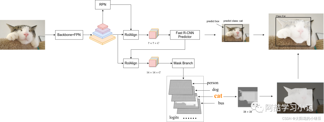
As shown in the figure above, through the Fast R-CNN branch, we can obtain the final predicted target bounding box information and category information. Next, the target bounding box information is provided to the Mask branch to predict the logits information for that target; then, based on the category information provided by the Fast R-CNN branch, we extract the mask information from logits corresponding to that category, which is the predicted mask information for that target (shape 28x28, with values between 0 and 1 due to the sigmoid activation function). We then use bilinear interpolation to scale the mask to the predicted target bounding box size and place it in the corresponding area of the original image. Finally, by setting a threshold (default is 0.5), we convert the mask into a binary image, for example, regions with predicted values greater than 0.5 are set as foreground, and the remaining regions are set as background. Now, for each predicted target, we can draw the bounding box information, category information, and target mask information on the original image.

This concludes the content on Mask R-CNN. The end, confetti.