Source: Big Data DigestThis article is approximately 4800 words, suggested reading time 10 minutes.

This article introduces a code simulation of playing Blackjack, transitioning from a naive strategy to deep learning.

Blackjack, also known as 21, originated in France and has a long history that has spread worldwide.With the development of the Internet, Blackjack has entered the online era, and it can now be found in casinos around the world. The game is played by 2 to 6 people using a standard deck of 52 cards, excluding jokers. The goal of the players is to have a hand value that does not exceed 21 while being as high as possible.A programmer on Medium has attempted to simulate playing Blackjack with code. After experimenting with a naive strategy, he shifted his focus to deep learning. Let’s take a look.Last time, we developed code to simulate playing Blackjack and discovered key factors that lead to winning in such games. Let’s quickly review:

1. The casino has the advantage of requiring Blackjack players (based on incomplete information) to draw cards before the dealer, which exposes players to the risk of busting (bust, when a player’s total exceeds 21). Some players may even bust before the dealer has drawn any cards.

2. When a player’s total is between 12 and 16 and is lower than the dealer’s total, it is particularly dangerous (the player risks busting when drawing the next card). In this case, if the dealer’s final total is high, the player must either continue to draw or stand. The diagram below clearly shows that when the total is in the range of 12 to 16, the player’s chances of winning are the lowest (we call this the “valley of despair”).

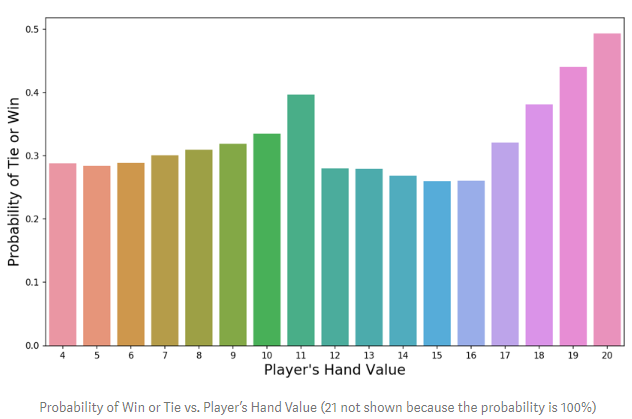
The probability of winning or tying changes with the total value of the player’s hand (a total of 21 guarantees a win, with a probability of 1).

3. Finally, we found that the naive strategy of “only drawing when there is no risk of busting” significantly increases the chances of defeating the casino, as this strategy shifts the risk of busting entirely onto the casino.

If you are not familiar with the game of Blackjack, you can refer to my previous article, which explains how to play and the corresponding rules.Article link:

https://towardsdatascience.com/lets-play-blackjack-with-python-913ec66c732f _blank

Can Deep Learning Do Better?The main purpose of this article is to determine whether deep learning can find a better strategy than the naive one mentioned above. We will:

1. Use the Blackjack simulator we developed last time to generate data (with minor adjustments to make it more suitable for training algorithms).

2. Code and train a neural network to play Blackjack (in optimal conditions).

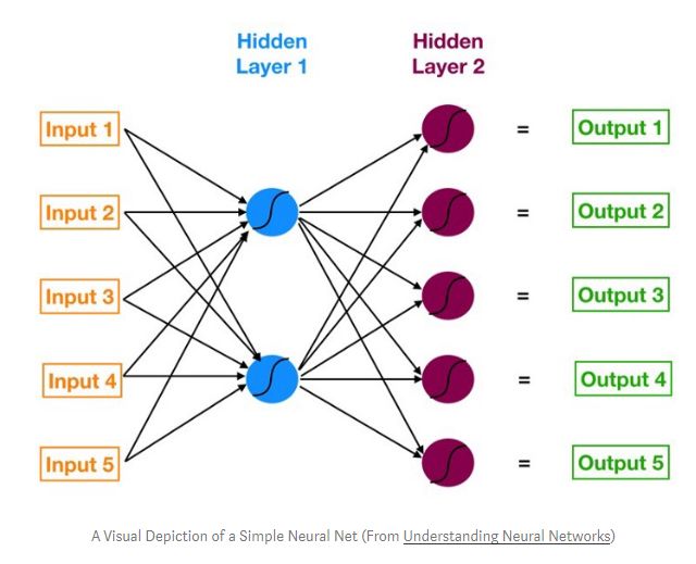
Illustration of a simple neural network

Before we enter the training process, let’s quickly discuss the pros and cons of using neural networks. Neural networks are highly flexible algorithms—like soft clay, they can self-adjust or make minor transformations to adapt to different datasets. They can easily handle more rigid problems like linear regression. Furthermore, network layers and neurons can learn nonlinear relationships hidden within the data.However, this versatility comes at a cost, as neural networks are black boxes. Unlike regression, where we can understand how the model makes decisions by examining regression coefficients, neural networks lack this transparency. Additionally, neural networks are at risk of overfitting, meaning they fit the data too closely and cannot generalize well to new samples. While these shortcomings are not enough to abandon neural networks, they are worth keeping in mind and designing safeguards against.Generating Training DataBefore training the neural network, we first need to clarify how to construct the training data, so that the resulting model is meaningful.What do we want to predict? In my opinion, we have two candidate parameters for our target variable:

1. The probability of losing the game. In this case, we may want the model to tell us the likelihood of failure. Again, this is only useful if we can increase or decrease the stakes, which is not applicable in Blackjack.

2. In fact, we would prefer our neural network to provide the correct action, whether to draw or stand. Therefore, our target variable should be “whether to draw or stand”.

I spent some time figuring out the best way to analyze the target variable. Here’s how I found it.We need a method to let the neural network know whether a given action is correct. This method does not need to be infallible; it just needs to be broadly correct. Therefore, I determined that the method for judging whether a given action is correct is to simulate a game of Blackjack: deal cards to the player and dealer, check if anyone has reached 21, decide on a draw action (draw or stand), and simulate the game until the end while recording the results. Since the simulated player makes only one decision at a time, we can evaluate the quality of that decision based on their win or loss:

• If the player draws and wins, then drawing (Y=1) is the correct decision.
• If the player draws but loses, then standing (Y=0) is the correct decision.
• If the player stands and wins, then standing (Y=0) is the correct decision.
• If the player stands but loses, then drawing (Y=1) is the correct decision.

We train the model based on this rule, with the output being a prediction for whether to draw or stand. The code this time is quite similar to last time, so I won’t go into detail here.GitHub link:

https://github.com/yiuhyuk/blackjack

The main functionalities of the code include:

1. The dealer’s upcard (the other card is face down)

2. The total value of the player’s hand

3. Whether the player has an Ace

4. The player’s decision (to draw or stand)

The target variable is the correct decision defined by the above logic.Training the Neural NetworkOur neural network will use Keras (an open-source neural network library). First, let’s look at the module imports:

from keras.models import Sequential
from keras.layers import Dense, LSTM, Flatten, Dropout

Next, we build the input variables for training the neural network. The variable feature_list is a list of names of features (X variables) that includes the ones mentioned above. The dataset model_df stores all the data generated by the Blackjack simulator.

# Set up variables for neural net
feature_list = [i for i in model_df.columns if i not in
               ['dealer_card','Y','lose','correct_action']]
train_X = np.array(model_df[feature_list])
train_Y = np.array(model_df['correct_action']).reshape(-1,1)

The code for instantiating and training the neural network is actually quite simple. The first line creates a sequential neural network, which is a linear stack of multiple network layers. The following code adds layers to our model one by one (where Dense defines the simplest network layer, which is a bunch of neurons), with the numbers 16 and 128 indicating the number of neurons.For the final layer, we need to choose an activation function. This function transforms the raw output of the neural network into something we can understand. There are two important points about the final layer: first, it contains only one neuron because we are predicting between two possible outcomes (a binary classification problem); second, we use the sigmoid activation function because we want our neural network to predict whether to draw (Y=1) or stand (Y=0), or in other words, we want to know the probability that the correct action is to draw.The last two lines of code tell our neural network what kind of loss function to use (binary crossentropy is a loss function used for classification models with probability outputs) and adjust the model to fit our data. I didn’t spend much time tuning the number of layers or neurons, but if you want to try my code, I think this could be a direction for model improvement.

# Set up a neural net with 5 layers
model = Sequential()                         # line 1
model.add(Dense(16))
model.add(Dense(128))
model.add(Dense(32))
model.add(Dense(8))
model.add(Dense(1, activation='sigmoid'))    # final layer
model.compile(loss='binary_crossentropy', optimizer='sgd')
model.fit(train_X, train_Y, epochs=20, batch_size=256, verbose=1)

Checking Model PerformanceA quick way to determine if our model is valuable is to use the ROC curve.Please check the link:

https://towardsdatascience.com/roc-curves-and-the-efficient-frontier-7bfa1daf1d9c）

The ROC curve can tell us how the model performs when weighing benefits (True Positive Rate) against costs (False Positive Rate)—the larger the area under the curve, the better the model performs.The following diagram shows the ROC curve of our Blackjack neural network—this seems significantly better than random guessing (red dashed line). The area under the curve, AUC, reaches 0.73, which is clearly higher than the AUC of random guessing (0.5).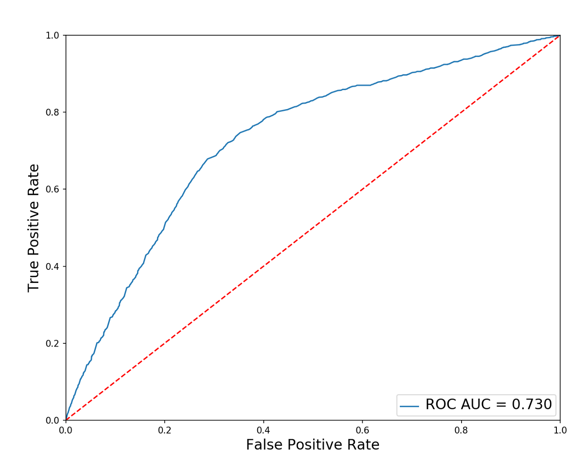

ROC curve of the Blackjack neural network

I used the training data to draw the ROC curve. Typically, we want to use validation or test data to plot it, but in this case, we know that as long as our sample size is large enough, it is representative of the whole (assuming the rules of Blackjack remain unchanged). We can also expect our model to have good generalization capabilities (any new data will have the same basic statistical characteristics as our training data).It’s Time to Shine!Before our neural network officially starts playing Blackjack, we need to give it a decision rule. Remember, the sigmoid activation function in the last layer of the neural network will convert the output into the probability of “the correct action is to draw.” Therefore, we need a decision rule that determines whether to draw based on this probability.The following function is used to determine this decision rule. The model_decision function makes predictions based on the input features required by the neural network and compares the prediction with a predefined threshold to decide whether to draw. Here I set the threshold at 0.52 because, from previous attempts, we found that busting is the greatest risk faced by Blackjack players. Thus, setting 0.52 as the threshold for drawing will slightly reduce the likelihood of the model choosing to draw, thereby also reducing the risk of busting.

def model_decision(model, player_sum, has_ace, dealer_card_num):
   input_array = np.array([player_sum, 0, has_ace,
                           dealer_card_num]).reshape(1,-1)
   predict_correct = model.predict(input_array)
   if predict_correct >= 0.52:
       return 1
   else:
       return 0

Now we need to integrate the above function into the code for deciding whether to draw. So when we need to decide whether to draw, the neural network will make a decision based on the dealer’s upcard, the total value of the player’s hand, and whether the player has an Ace.Our Model Performs Well!Finally, let’s compare the performance of the neural network model with the naive strategy model and the random model. A few points are worth noting:

• I simulated about 300,000 games of Blackjack for each strategy type (neural network, naive, random).
• The naive strategy only draws when the bust probability is zero (draw when the player’s total is less than 12, stand when the total is 12 or more).
• The random strategy refers to choosing to draw based on the result of a coin flip; if heads, draw, otherwise stand. If a draw is chosen and there is no bust, continue to flip the coin and repeat the process.

Let’s see if the neural network has found a better strategy. The table below shows the results distribution for various strategy types. From this, I have two findings: first, our neural network lost in less than half of the games (49%). While it is hard to say whether we would ultimately win, this is quite a good result for a game with fixed odds; second, the neural network does not actually lead to more wins than the naive strategy, but instead is able to force ties with the opponent more frequently.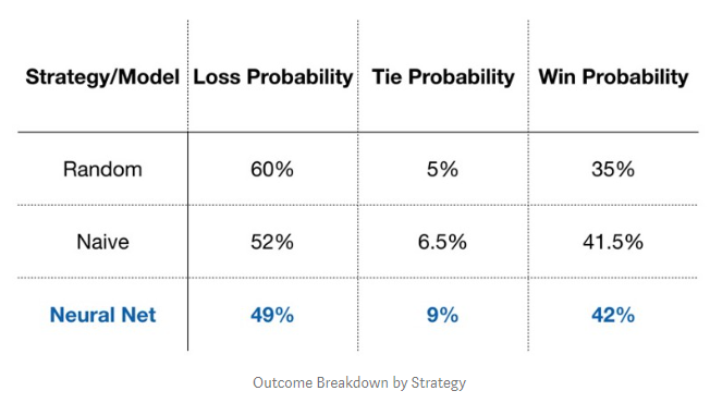

Results of various strategy types

We can also observe how different strategies perform on some important features (the dealer’s upcard and the total value of the player’s hand). First, let’s look at how the dealer’s upcard affects the probability of winning or tying for our three strategies. In the diagram below, if the dealer’s upcard is low, the performance of the neural network is not much different from the naive strategy. However, when the dealer’s upcard is high (7 or more), the neural network’s performance is significantly better.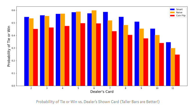

The probability of winning or tying changes with the dealer’s upcard value (the longer the bar, the greater the probability!)

We can also examine how the probability of winning or tying changes with the total value of the player’s initial hand. The results look great; regardless of the total value of the player’s initial hand, our neural network performs as well as or even better than the other two strategies. In contrast, the naive strategy performs even worse than the random strategy in the valley of despair (when the player’s initial hand total is between 12 and 16). There is no doubt that the neural network has better performance.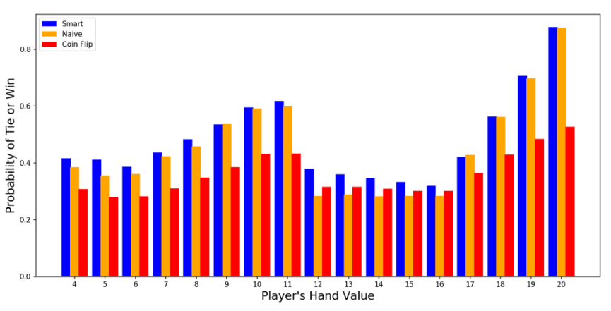

The probability of winning or tying changes with the total value of the player’s initial hand (the longer the bar, the greater the probability!)

The following diagram illustrates how the neural network outperforms the naive strategy. According to our code, the naive strategy is unwilling to take risks and draw even when the player faces a minimal risk of busting. On the other hand, when the player’s initial hand total is 12, 13, 14, or 15, the neural network is more inclined to draw. This subtle change in decision-making and the ability to calculate risks seem to be the reasons why the neural network outperforms the naive strategy.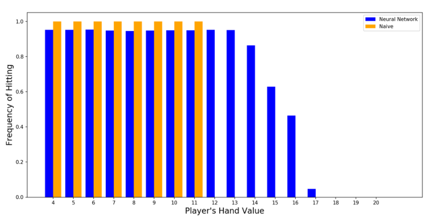

The trend of neural network versus naive strategy in choosing to draw based on the player’s initial hand total

We can observe what the neural network does to try to improve our naive strategy (minimizing losses to the casino) when the player’s hand total is between 12 and 16. When the dealer’s upcard is high (8, 9, or 10), the neural network is very inclined to draw. But even when the dealer’s upcard is low (for example, 3), the neural network still chooses to draw 60% of the time because it considers all available features when making decisions. Therefore, we cannot easily distill its decision-making into simple heuristics.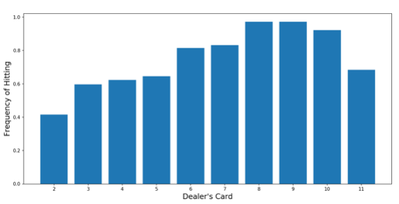

The frequency of the neural network choosing to draw changes with the dealer’s upcard

ConclusionI hope this article provides a suitable explanation for using machine learning to assist decision-making in life. When training your own models, keep the following points in mind (whether decision trees, regression, or neural networks):Is it possible to solve the current problem by predicting the target variable? It is crucial to ensure you have chosen the correct prediction target before starting to collect data and build a model.What differences might exist between real data and training data? If there is a significant discrepancy between the two, then the network model may not be the right answer to the problem. At the very least, we must be aware of this and take measures such as regularizing the model and rigorously (and honestly) validating and selecting a benchmark for the test set.If you do not understand how decisions are formed, you cannot rationally check the model’s decisions against test data that was not included during the training process.Finally, I would like to say a few words about the game of Blackjack. I may not discuss gambling topics for a while (I have too many topics I want to explore). But if anyone is interested in continuing to explore this topic (whether or not using my code), consider some interesting extensions:

1. Try to improve the model through more optimized neural network structures, or add code for splitting Aces (which I did not build into the original simulator), or choose a better feature set than the basic one I used.

2. Add the ability to calculate the total point value and observe how it affects model performance with one deck versus six decks (Las Vegas standard).

Link:

https://towardsdatascience.com/teaching-a-neural-net-to-play-blackjack-8ec5f39809e2

Editor: Yu TengkaiProofreader: Wang Xin