This article is a translated note of the Stanford University CS231N course, authorized for translation and publication by Professor Andrej Karpathy of Stanford University. The Big Data Digest work is prohibited from being reproduced without authorization; specific requirements for reproduction can be found at the end of the article.

Registration is open!

Machine Learning training registration has begun!
Top instructors and course design
Theory combined with practice
Plus five major benefits available
Click "Read the original text" at the end for details

Translation: Han Xiaoyang & Long Xincheng

Editor’s Note: This article is the second series we bring to readers from the Stanford course articles on the topic of the Stanford Deep Learning and Computer Vision Course, covering the third and fourth issues. The content is from the Stanford CS231N series, intended for interested readers to experience and learn.

Video translations of this course are also in progress and will be released soon; stay tuned!

The Big Data Digest will continue to publish translations and videos, freely sharing them with readers.

We welcome more interested volunteers to join us for learning and exchange. All translators are volunteers; if you are like us, capable and willing to share, please join us. Reply “Volunteer” in the Big Data Digest backend to learn more.

The Stanford University CS231N course is a classic tutorial in deep learning and computer vision, highly rated in the industry. Previously, some friends in China did some sporadic translations; to share high-quality content with more readers, the Big Data Digest has conducted a systematic and comprehensive translation, with subsequent content to be released gradually.

Due to the limitations of the WeChat backend code editor, we have used image insertion to display the code; click on the image to view a clearer version.

Meanwhile, the first series of Stanford courses that the Big Data Digest has previously authorized, the Stanford University CS224d course on Machine Learning and Natural Language Processing, has completed eight sessions. We will continue to push subsequent notes and course videos every Wednesday; please pay attention.

Reply “Stanford” to download the PDF version of notes for the third and fourth issues of CS231N

Also obtain materials related to another series of Stanford courses, CS224d, on deep learning and natural language processing

Additionally, for readers interested in further learning and exchange, we will organize study exchanges through QQ groups (given the limitation of the number of people on WeChat).

Long press the following QR code to jump directly to the QQ group

Or join the group with the group number 564538990

◆ ◆ ◆

1.Introduction

In the previous section of the deep learning and computer vision series (3) _ Linear SVM and SoftMax Classifier (due to WeChat editing length limitations, the content of the third issue is only provided as an overview here; please reply “Stanford” to download the content of the third issue notes), two concepts crucial for image recognition were mentioned:

1. The score function used to map raw pixel information to different category scores.

2. The loss function used to evaluate the effectiveness of parameter W (assessing the degree of fit between the scores of each category under this parameter and the actual scores).

For linear SVM, we have:

With suitable parameter W, the predicted results obtained from raw pixels align very closely with the actual results, resulting in a very small value for the loss function.

This section will discuss how to obtain the suitable parameter W that minimizes the value of the loss function, which is the optimization process.

◆ ◆ ◆

2. Visualizing the Loss Function

The loss functions we see in computer vision are usually defined in very high-dimensional spaces (for example, in the CIFAR-10 case, a linear classifier’s weight matrix W is 10 x 3073 dimensions, totaling 30730 parameters -_-||), making it very difficult for humans to directly “see” its shape/variation. However, clever students always find ways to visualize the loss function to some extent. For instance, we can project high dimensions onto a vector/direction (1D) or a plane (2D) to intuitively “observe” some changes.

For example, we can find a line in the weight matrix W (for example, in CIFAR-10, there are 30730 parameters) and calculate the variation of the loss function along this line for different values of a. Specifically, we find a vector W1 (which must have the same dimension as W, so that W1 can represent a direction in W’s dimensional space), and then for different values of a, we calculate L(W + aW1). If a is sufficiently dense, we can depict the changes of the loss function along this direction to some extent.

Similarly, if we have two directions W1 and W2, we can define a plane, then take different values of a and b to calculate L(W + aW1 + bW2), allowing us to roughly sketch the changes in the loss function on this plane.

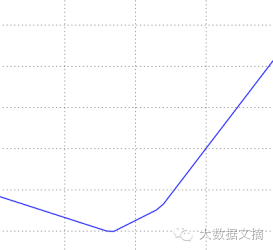
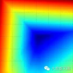
Using the above method, we plotted three graphs below. The top graph shows the loss function’s variation curve (the higher the value, the larger); the middle and bottom graphs show the loss function’s variation on a sample image (blue indicates low loss, red indicates high loss), with the middle graph calculated based on one image sample, and the bottom graph showing the average loss results calculated over 100 images. It is evident that the curve’s lowest point along the linear direction represents the minimum loss value, while the surface presents a bowl-shaped graph, with the bowl’s bottom being where the loss function takes its minimum value.

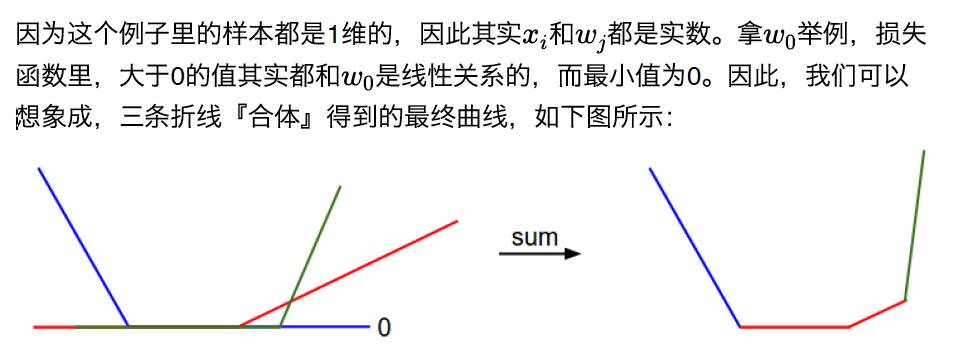
From a mathematical perspective, we attempt to explain how the above concave curve is generated. For the i-th sample, we know its loss function value is:

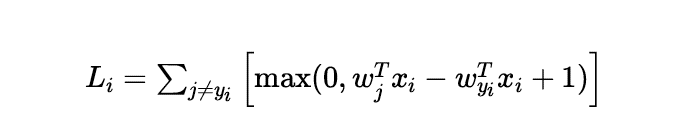
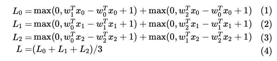
The loss function values across all samples are the average of their loss function values (max(0,-), hence the minimum value is 0). For better understanding, we assume there are 3 samples in the training set, all one-dimensional, and there are 3 categories in total. Therefore, the SVM loss (temporarily ignoring the regularization term) can be expressed as follows:

◆ ◆ ◆

3. Optimization

In our current problem, “optimization” refers to finding the parameters that minimize the loss function. If you have seen or understand <span>convex optimization</span>, the method we will introduce next may seem too simple and a bit <span>primitive</span>, but let’s not forget that we will later deal with the loss function of neural networks, which is not a convex function, so we will still take it step by step to see how to implement the optimization problem.

3.1 Strategy 1: Random Search (Not Very Practical)

Starting with a simple method, we know that once we have the parameters, we can calculate the loss function to assess the suitability of the parameters. Therefore, the most straightforward and brute-force method is to try many parameters and select the one that minimizes the loss function as the final one. The code is, of course, very simple, as follows:

# Assume X_train is the training set (e.g., 3073 x 50,000)
# Assume Y_train is the category results (e.g., a 1D array of 50,000)

bestloss = float("inf") # Initialize a maximum float value
for num in xrange(1000):
  W = np.random.randn(10, 3073) * 0.0001 # Randomly generate a set of parameters
  loss = L(X_train, Y_train, W) # Calculate the loss function
  if loss < bestloss: # Compare with the best result found so far
    bestloss = loss
    bestW = W
  print 'in attempt %d the loss was %f, best %f' % (num, loss, bestloss)

# prints:
# in attempt 0 the loss was 9.401632, best 9.401632
# in attempt 1 the loss was 8.959668, best 8.959668
# in attempt 2 the loss was 9.044034, best 8.959668
# in attempt 3 the loss was 9.278948, best 8.959668
# in attempt 4 the loss was 8.857370, best 8.857370
# in attempt 5 the loss was 8.943151, best 8.857370
# in attempt 6 the loss was 8.605604, best 8.605604
# ... (truncated: continues for 1000 lines)

After a series of random trials and searches, we will obtain the best parameter W from the experimental results, and then test its effectiveness on the test set:

# Assume X_test is [3073 x 10000], Y_test is [10000 x 1]
scores = Wbest.dot(Xte_cols) # 10 x 10000, calculate category scores
# Find the highest score as the result
Yte_predict = np.argmax(scores, axis = 0)
# Calculate accuracy
np.mean(Yte_predict == Yte)
# Returns 0.1555

The parameters W obtained from random search yielded an accuracy of 15.5% on the test set; with a total of 10 categories, our random guessing should yield an accuracy of about 10%, so it seems a bit higher, but… as you can see… this accuracy… is practically unusable in real applications.

3.2 Strategy 2: Random Local Search

The previous strategy was entirely blind searching, making it nearly impossible to find the global optimal result. Its biggest drawback is that the next search is completely random, without any guiding direction. However, with some thought, we can come up with an optimized version based on the previous strategy, called “random local search”.

This strategy means that we do not randomly generate a parameter matrix W each time; instead, we search for better nearby parameters based on the current parameter W, and if we find a better W, we replace the current W with the new one and continue to search in the vicinity. This process can be imagined as being on a mountain; when we want to descend, we stretch our foot to explore nearby to find a position lower than our current one, then step forward, and repeat this process until we reach the bottom.

From the coding perspective, this process is actually about taking the current W, experimenting with it, and adding a small perturbation to W, then checking if the loss function is lower than the current one. If it is, we replace the current W, as shown in the code below:

W = np.random.randn(10, 3073) * 0.001 # Initialize weight matrix W
bestloss = float("inf")
for i in xrange(1000):
  step_size = 0.0001
  Wtry = W + np.random.randn(10, 3073) * step_size
  loss = L(Xtr_cols, Ytr, Wtry)
  if loss < bestloss:
    W = Wtry
    bestloss = loss
  print 'iter %d loss is %f' % (i, bestloss)

After making this small adjustment, we tested the same test set again, and the accuracy improved to 21.4%. Although it is still far from practical applications, it is just a slight improvement over the previous method.

However, there is still a problem: testing the loss function of nearby points is a very time-consuming task. Is there a way to directly find the direction we should iterate in?

3.3 Strategy 3: Gradient Descent

The previous strategy was very time-consuming and computationally intensive. What we have been doing is trying to find the most suitable direction to descend based on the current position. Let’s return to our assumed scenario: if we are at the top of a mountain and want to descend as quickly as possible, what would we do? We might look around and find the steepest direction, take a small step, and then find the steepest descent direction from our current position, and repeat this process…

The steepest direction mentioned here corresponds to the mathematical concept of “gradient”. This means we do not need to “probe” the steepness around; instead, we can calculate the gradient of the loss function to directly obtain this direction.

We know that in a single-variable function, the slope/derivative at a point represents the direction of maximum change. For multivariable cases, the gradient is an extension of this situation, where the variables are no longer one but multiple, and the “gradient direction” we calculate is also a multidimensional vector. As everyone knows, the mathematical expression for calculating the “gradient/derivative” of a 1D function is as follows:

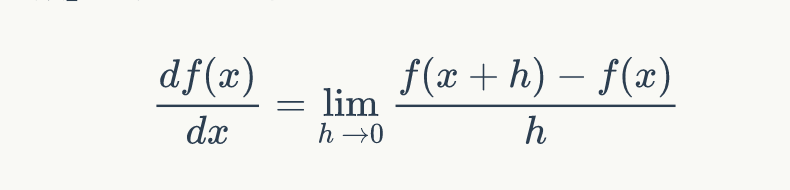
For multivariable cases, we need to obtain the “partial derivatives” in each direction and combine them to form our gradient vector.

We can illustrate this process with a few diagrams:

◆ ◆ ◆

4. Calculating Gradients

There are two methods for calculating gradients:

1. Slower but easier numerical gradient

2. Faster but more error-prone analytical gradient

4.1 Numerical Gradient

Based on the derivative solving formula mentioned above, we can obtain the numerical gradient calculation method. Below is a simple piece of code to compute the gradient at a given function f and a vector x:

def eval_numerical_gradient(f, x):
  """
  A basic algorithm to compute the gradient of f at point x
  - f is a function with parameter x
  - x is a numpy vector
  """

  fx = f(x) # Calculate the function value at the original point
  grad = np.zeros(x.shape)
  h = 0.00001

  # Calculate for each dimension of x
  it = np.nditer(x, flags=['multi_index'], op_flags=['readwrite'])
  while not it.finished:

    # Calculate the function value at x+h
    ix = it.multi_index
    old_value = x[ix]
    x[ix] = old_value + h # Add h
    fxh = f(x) # Calculate f(x + h)
    x[ix] = old_value # Restore previous function value

    # Calculate the partial derivative
    grad[ix] = (fxh - fx) / h # Slope
    it.iternext() # Move to the next dimension

  return grad

The method in the code is simple; for each dimension, we add a small h to the original value and then calculate the partial derivative in that dimension/direction, finally assembling them together to obtain the gradient grad.

4.1.1 Tips for Actual Calculations

If we look closely at the derivative solving formula, we will find that mathematically, h should approach 0, but in practice, we only need to take a sufficiently small number (like 1e-5) as h. Therefore, to calculate the partial derivative accurately, we should take h to be small enough to avoid numerical computation issues while still being sufficiently small. Additionally, in actual computations, we often use another formula more frequently:

Now let’s try the above formula on the CIFAR-10 dataset:

def CIFAR10_loss_fun(W):
  return L(X_train, Y_train, W)

W = np.random.rand(10, 3073) * 0.001 # Random weight vector
df = eval_numerical_gradient(CIFAR10_loss_fun, W) # Calculate gradient

The calculated gradient (to be precise, the direction of the gradient indicates the direction of maximum increase of the function, while the negative gradient indicates the direction of descent) tells us what direction we should “descend”. We then take small steps along that direction:

loss_original = CIFAR10_loss_fun(W) # Loss at the original point
print 'original loss: %f' % (loss_original, )

# How far should we step? Let's try some step sizes
for step_size_log in [-10, -9, -8, -7, -6, -5,-4,-3,-2,-1]:
  step_size = 10 ** step_size_log
  W_new = W - step_size * df # New weights
  loss_new = CIFAR10_loss_fun(W_new)
  print 'for step size %f new loss: %f' % (step_size, loss_new)

# Output:
# original loss: 2.200718
# for step size 1.000000e-10 new loss: 2.200652
# for step size 1.000000e-09 new loss: 2.200057
# for step size 1.000000e-08 new loss: 2.194116
# for step size 1.000000e-07 new loss: 2.135493
# for step size 1.000000e-06 new loss: 1.647802
# for step size 1.000000e-05 new loss: 2.844355
# for step size 1.000000e-04 new loss: 25.558142
# for step size 1.000000e-03 new loss: 254.086573
# for step size 1.000000e-02 new loss: 2539.370888
# for step size 1.000000e-01 new loss: 25392.214036

4.1.2 Details on Iteration

If you look closely at the code above, you will notice that we set the step_size to be negative. Indeed, when we update the weight W, we subtract a small value in the direction of the gradient so that the loss function can decrease.

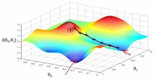
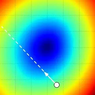
4.1.3 About the Step Size for Iteration

After calculating the gradient, we have determined the direction of maximum change (the negative gradient is the direction of descent), but it does not inform us how far we should step in that direction. The correct choice of iteration step size (sometimes also called learning rate) is one of the most important (and often frustrating) parameters to set during training. For instance, if we want to descend the fastest, we can sense the steepest direction but do not know how large a step we should take. If we take very small steps, we can indeed decrease at each step, but the pace is too slow! Conversely, if we take very large steps (imagine having very long legs -_-||), you might accidentally leap over the foot of the mountain and land on another mountain’s slope…

The following image describes and explains this situation:

4.1.4 Efficiency Issues

If you look back at the program for calculating the numerical gradient, you will find that the computational complexity is basically linear with respect to the number of parameters. What does this mean? In our CIFAR-10 example, we have a total of 30730 parameters, so we need to compute the loss function 30731 times for each iteration. This issue becomes even more severe in neural networks, where there can be millions of parameters between two layers of neurons, making computation very time-consuming… and humans have to wait for the results with tears…

4.2 Analytical Gradient Calculation

While numerical gradients are very easy to implement, we can see from the formula that gradients are essentially approximations (after all, you cannot take h to be extremely small), and this is a very time-consuming algorithm. The second method for calculating gradients is the analytical method, which allows us to directly obtain a formula for the gradient (substituting it in is very fast), but unlike numerical gradient methods, this approach is more prone to errors. Thus, clever students have come up with a method: we can first calculate both the analytical and numerical gradients, then compare the results and correct them, and once we confirm that our analytical gradient implementation is correct, we can boldly proceed with the analytical method (this process is called gradient checking).

Let’s take the loss function of a sample point’s SVM as an example:

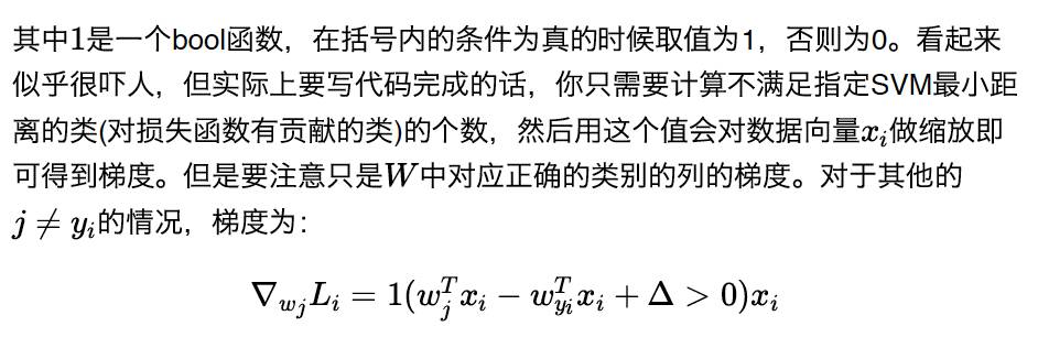
Once we obtain the expression for the gradient, calculating the gradient and adjusting weights becomes very straightforward and simple. Mastering how to calculate gradients under the loss expression is a very important skill that runs through the entire training implementation process of neural networks; this content will be discussed in detail next time.

◆ ◆ ◆

5. Gradient Descent

Once we have a way to calculate gradients, the process of using the gradient to update existing weight parameters is called “gradient descent”. The pseudocode is actually as follows:

while True:
  weights_grad = evaluate_gradient(loss_fun, data, weights)
  weights += - step_size * weights_grad # Gradient descent updates parameters

This simple loop is essentially the core of many neural network libraries. Of course, there are other ways to implement optimization (such as L-BFGS), but gradient descent is indeed the most widely used and relatively stable method for optimizing the loss functions of neural networks.

5.1 Mini-batch Gradient Descent

In large applications (such as ILSVRC), training data can be in the millions or tens of millions. Therefore, calculating the loss function for every sample in the entire training dataset to complete parameter iterations is very time-consuming. A commonly used alternative method is to sample a subset to calculate the gradient. Most cutting-edge neural network structures do this; for example, ConvNets use 256 images as a batch to complete parameter updates. The parameter update code is as follows:

while True:
  data_batch = sample_training_data(data, 256) # Sample 256 samples as a batch
  weights_grad = evaluate_gradient(loss_fun, data_batch, weights)
  weights += - step_size * weights_grad # Parameter update

This is possible because the training data are actually related. To simplify this problem, consider that if there are 120,000 images in ILSVRC, and we only have 1000 different images, duplicating them 1200 times will yield similar loss function results as averaging over 120,000 images. Of course, in practice, we rarely encounter such repeated situations, but the gradient on a subset (mini-batch) of the original data is also a good approximation of the overall gradient. Therefore, computing and updating parameters only on the mini-batch will lead to much faster convergence.

An extreme case of the above algorithm is if our mini-batch contains only one image. This process becomes “Stochastic Gradient Descent (SGD)”. In practice, this is not very common; the reason is that vectorization allows calculating 100 images at once to be much faster than calculating one image 100 times. Thus, even though SGD is defined as using the gradient from one image to approximate the global gradient, many times when people refer to SGD, they actually mean mini-batch gradient descent, treating one batch as one sample. Additionally, it should be noted that some may ask if the batch size itself is a parameter that needs to be experimented with; what is a good batch size? In practical applications, we rarely use cross-validation to select this parameter. Generally speaking, we set this value based on our memory constraints, typically around 100.

◆ ◆ ◆

6. Summary

• Imagine the values of the loss function across parameters as the height of the mountain we are on. To minimize the loss function, we essentially need to “find a way down the mountain”.

• Our strategy for descending is to take small steps; as long as we move down each time, we will eventually reach the bottom of the mountain.

• The gradient corresponds to the direction of maximum change of the function, and the negative gradient direction is our descent direction, where we find the steepest way down.

• Our step size (also called learning rate) affects our convergence speed (the speed of descent); if the steps are too large, we might leap over the lowest point and land on another high point.

• We use mini-batch methods, calculating and updating parameters on a small subset of samples to reduce computation and speed up convergence.

About Reproduction

For reproduction, please prominently indicate the author and source at the beginning (transferred from: Big Data Digest | bigdatadigest) and place the prominent QR code of Big Data Digest at the end of the article. Articles without original identification should be edited according to reproduction requirements and can be directly reproduced. After reproduction, please send us the reproduction link; for articles with original identification, please send [Article Name - Public Account Name and ID for Authorization] to apply for whitelist authorization. Unauthorized reproduction and adaptation will be legally pursued. Contact email: [email protected].

◆ ◆ ◆

Big Data Articles Stanford Deep Learning Course

Reply “Volunteer” in the Big Data Digest backend to learn how to join us

Column Editor

Project Management

Content Operations: Wei Zimin

Overall Coordination: Wang Decheng

Previous Excellent Articles Recommended, click the image to read

[Another Heavyweight] Translation Authorization Obtained Again, Stanford CS231N Deep Learning and Computer Vision

Stanford Deep Learning Course Episode 7: RNN, GRU, and LSTM

Stanford CS231N Deep Learning and Computer Vision Episode 2: Image Classification and KNN