This article is a Chinese version of the Stanford University CS231N course notes, authorized for translation and publication by Professor Andrej Karpathy of the Stanford course. This is a work by Big Data Digest, and unauthorized reproduction is prohibited. For specific requirements for reproduction, please see the end of the article.

Machine Learning Online Training Starts on August 30!

Machine Learning Training Registration is Now Open!
Top Instructor Course Design
Theory Combined with Practice
Five Major Benefits Provided
Click "Read the Original" at the end of the article for details

Translation: Han Xiaoyang & Long Xincheng

Editor’s Note:This article is the second series of our articles for readers on the Stanford course, the sixth installment of the [Stanford Deep Learning and Computer Vision Course]. The content is from the Stanford CS231N series, intended for interested readers to experience and learn.

Video translations for this course are also underway and will be released soon, so stay tuned!

Big Data Digest will continue to release translations and videos, sharing them for free with all readers.

We welcome more interested volunteers to join us for communication and learning. All translators are volunteers; if you are capable and willing to share like us, please join us. Reply “Volunteer” in the backend of Big Data Digest to learn more.

The Stanford CS231N course is a classic tutorial in deep learning and computer vision, highly regarded in the industry. Previously, some friends in China had done some sporadic translations. To share high-quality content with more readers, Big Data Digest has conducted a systematic and comprehensive translation, and subsequent content will be released gradually.

Due to the limitations of the WeChat backend code editor, we have adopted an image insertion method to present the code; click on the image for a clearer view.

Meanwhile, Big Data Digest has previously obtained authorization for the first series of Stanford coursesStanford University CS224d Course [Machine Learning and Natural Language Processing], which has completed eight sessions. We will continue to push subsequent notes and course videos every Wednesday, so please pay attention.

Reply “Stanford” to download related materials for the CS231N series

Also obtain related materials for another Stanford series courseCS224d on deep learning and natural language processing

Additionally, for readers interested in further learning and communication, we will organize learning exchanges through QQ group (due to the limitation of WeChat group members).

Long press the following QR code to jump directly to the QQ group

Or join the group using the group number285273721

◆ ◆ ◆

Introduction

As we all know, deep learning and neural networks were initially designed inspired by the neurons of the human brain. Therefore, we will also explain the background from a biological perspective, of course, also paying tribute to the pioneers of neural network research.

◆ ◆ ◆

Neurons and Their Meaning

1. Neuron Activation and Connections

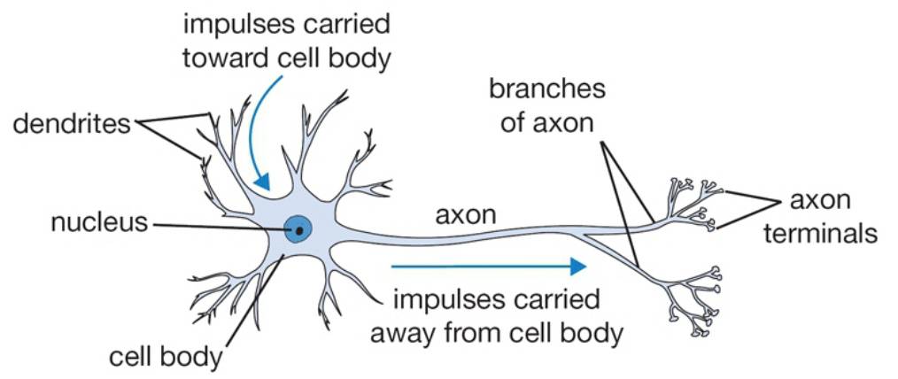
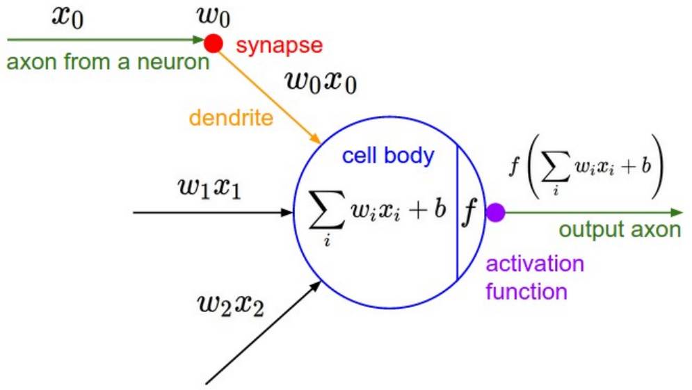
As we all know, the basic computational unit of the human brain is called a neuron. Modern biology shows that there are approximately 86 billion neurons in the human nervous system, and these numerous neurons are connected by about synapses. Below is a schematic diagram that roughly depicts the neurons in the human body and our simplified mathematical model. Each neuron receives signals from dendrites and transmits signals along an axon. Each neuron has many axons connected to the dendrites of other neurons. In the simplified computational model of the neuron on the right, signals are also transmitted along the axon (for example, ), then at the axon terminals, they are stimulated ( times) and become . We can understand this model as follows: in the process of signal transmission, synapses can control the strength of the signal transmitted to the next neuron (the weights in the mathematical model), and this strength can be learned. In the basic biological model, dendrites transmit signals to the neuron cell, and these signals are summed together; if the sum exceeds a certain threshold perceived by the neuron, the neuron is activated and transmits signals to the next neuron along the axon. In our simplified mathematical model, we assume there is an ‘activation function’ that controls the degree of stimulation of the summation result on the neuron, thereby controlling whether to activate the neuron and propagate signals backward. For example, the sigmoid function we use in logistic regression is an activation function because, for the input of the summation result, the sigmoid function will always output a value between 0 and 1, which we can consider as indicating the strength of the signal or the probability of the neuron being activated and transmitting signals.

Below is a simple program example that shows what a single neuron does during forward propagation:

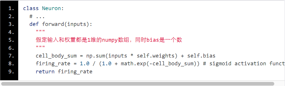A brief explanation: each neuron performs an inner product with the input and weights, adds a bias, and then passes through an activation function (such as the sigmoid function here), and finally outputs the result.

Special Note: Neurons in actual biological organisms are quite complex; for example, there are numerous types of neurons, each with different functions. The non-linear transformation of the activation function after summing signals is also much more complex than the functions simulated mathematically. The neural network modeled mathematically is just a very simplified model; if interested, you can read Material 1 or Material 2.

2. Classification Function of a Single Neuron

Taking the sigmoid function as an example of the neuron’s activation function, this might be somewhat familiar, as we emphasized this non-linear function in the logistic regression section, compressing input values into a probability value between 0 and 1. Through this non-linear mapping and set threshold, we can partition the space into areas corresponding to positive and negative samples. Corresponding back to the current neuron scenario, if we slightly personify, we can consider that neurons possess the ability to like (probability close to 1) and dislike (probability close to 0) certain spatial regions. This means that as long as the weights are adjusted correctly, a single neuron can perform linear segmentation of the space.

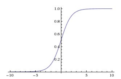
Binary Softmax Classifier

For detailed content on the Softmax classifier, please refer to the previous blog series. We denote as the sigmoid mapping function; thus, can be seen as the probability of belonging to a certain class in a binary classification problem 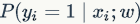. Of course, we can also obtain the probability for the opposite category as . Based on the knowledge mentioned in the previous blog, we can use cross-entropy loss as the loss function for this binary linear classifier, and the set of parameters obtained from optimizing the loss function can help us linearly segment the space and achieve binary classification. Of course, just like we saw in logistic regression, if the final predicted result y of the neuron is greater than 0.5, we would determine it belongs to this class; otherwise, it belongs to the other class.

Binary SVM Classifier

Similarly, we can set the max-margin hinge loss as the loss function, thus training the neuron to become a binary support vector machine classifier. For detailed content, please refer to the previous blog.

Explanation of Regularization

For the regularization loss function (whether SVM or Softmax), we can actually find corresponding explanations in the biological characteristics of neurons. We can view the role of the regularization term as the gradual fading/decay (gradual forgetting) of signals during the transmission process in the neuron because the role of the regularization term is to control the magnitude of the weights towards 0.

The function of a single neuron can be viewed as completing a binary classification (such as Softmax or SVM classifier)

3. Common Activation Functions

After each input and weight linear combination, it will pass through an activation function (also called a non-linear activation function), outputting after a non-linear transformation. In actual neural networks, there are several optional activation functions, and we will explain the most common ones one by one:

3.1 Sigmoid

• The sigmoid function is prone to saturation and terminate gradient propagation during actual gradient descent. Let me explain: as everyone knows, the backpropagation process relies on the computed gradient, which is the slope in a single-variable function. On the graph of the sigmoid function, it is evident that at the positions near 0 and 1 on the vertical axis (when the amplitude of the input signal is large), the slope approaches 0. Recalling the backpropagation process, the gradient we use for iteration is obtained by multiplying these intermediate gradient values, so if the intermediate local gradient values are very small, it will directly pull the final gradient result close to 0, meaning that the process of residual backpropagation is ‘killed’ due to the saturation of the sigmoid function. In an extreme case, if we do not initialize the weights appropriately at the beginning and use the sigmoid function for activation, it is very likely that all neurons will saturate to the point of being unable to learn, and the entire neural network will not be able to train.

• The output of the sigmoid function is not zero-centered, which is a troublesome issue because the output of each layer serves as the input for the next layer, and non-zero centering will directly affect gradient descent. Let’s illustrate this with an example: if the output results are not centered around 0, in an extreme case, all positive (for example, ), then the gradients backpropagated to will be either all positive or all negative (depending on the gradient of f). The consequence of this is that when the gradients obtained from backpropagation are used for weight updates, they do not change smoothly but instead exhibit a sawtooth-like abrupt change. Of course, it should be noted that this disadvantage is somewhat better than the first disadvantage; the first disadvantage leads to the neural network being unable to learn in many scenarios.

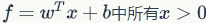
3.2 Tanh

The Tanh function is shown in the above image. It compresses input values to between -1 and 1; of course, it also has the first disadvantage mentioned for the sigmoid function, where neurons easily saturate with very large or very small input values. However, it alleviates the second disadvantage because its output is zero-centered. Therefore, in practical applications, the Tanh activation function is used more than the sigmoid.

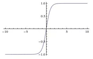
3.3 ReLU

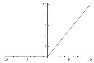
ReLU stands for Rectified Linear Unit, which has been widely used in recent years, as shown in the image above. It calculates 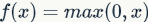for the input x; in other words, everything to the left of 0 is 0, and to the right is the line y=x.

It has its advantages and disadvantages:

Advantage 1: Experiments have shown that its use can significantly speed up the convergence of stochastic gradient descent compared to sigmoid and tanh. Interestingly, many say that this result is due to its linearity, unlike sigmoid and tanh, which are non-linear. The convergence speed comparison is shown in the following figure, where the convergence speed can be about 6 times faster:

Advantage 2: Compared to tanh and sigmoid activation neurons, computing gradients is much simpler!!! After all, it is linear.

Disadvantage 1: The ReLU unit has its drawbacks; during training, it is quite fragile and can sometimes die. For example, if a very large gradient flows through the ReLU unit, the result of the weight update may lead to the fact that no data points can activate it afterward. Once this happens, the gradients that should have been backpropagated through this ReLU will forever become 0. Of course, this is related to parameter settings, so we need to be particularly careful. For instance, if the learning rate is set too high, you may find that up to 40% of the ReLU units die during training. Therefore, we need to be cautious in setting the initial learning rate and other parameters to control this issue.

3.4 Leaky ReLU

As mentioned above, the weakness of the ReLU unit has led diligent ML researchers to try to fix this problem. They have done this by not allowing y to take the value of 0 for x<0; instead, it is set to a line with a very small slope (for example, a slope of 0.01). Therefore, f(x) becomes a piecewise function, for x<0, , ( is a very small constant), and for x>0, . Some researchers claim that this form of activation function helps them achieve better results, but it seems that it does not always have advantages over ReLU.

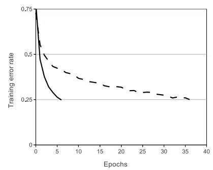
3.5 Maxout

There are also other activation functions that do not perform non-linear mapping on . A very popular activation function in recent years is Maxout (for detailed content, please refer to Maxout). In simple terms, it is a generalized version of ReLU and Leaky ReLU. For input x, Maxout neurons compute . Interestingly, if you look closely, you will find that both ReLU and Leaky ReLU are special forms of it (for example, for ReLU, you only need to set to 0). Therefore, Maxout neurons inherit the advantages of ReLU units without the concern of ‘dying’ easily. If we were to mention disadvantages, you can see that compared to ReLU, the computational load doubles because of the two linear mapping operations.

4 Summary of Activation Functions/Neurons

Above are the common types of neurons and activation functions we summarized. By the way, even if it seems feasible from the computational and training perspectives, in practical applications, we rarely mix different activation functions.

So how do we choose neurons/activation functions? Generally speaking, ReLU is still the most commonly used, but we do need to be cautious in setting the learning rate, and during training, we should periodically check the status of the neurons (whether they are still ‘alive’). Of course, if you are very concerned about neurons dying during training, you can try Leaky ReLU and Maxout. Well, let’s use sigmoid less often, and if you are interested, you can try tanh, but usually, its performance is not as good as ReLU/Maxout.

◆ ◆ ◆

Neural Network Structure

1. Hierarchical Connection Structure

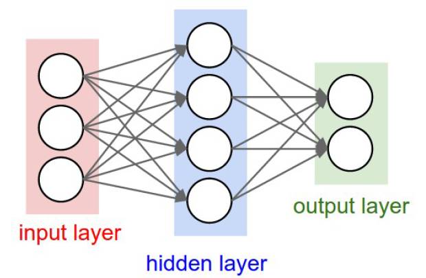
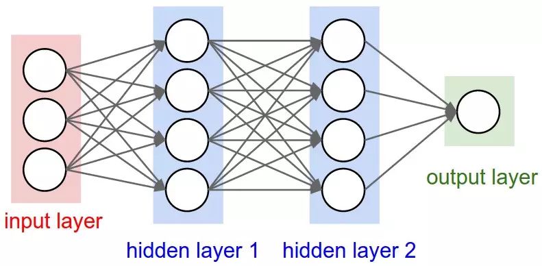
The structure of a neural network has been mentioned before; it is a unidirectional hierarchical connection structure, where each layer may have multiple neurons. To be more illustrative, the output of each layer will serve as the input data for the next layer; of course, this diagram must not have loops; otherwise, the data flow would be somewhat chaotic. Generally, there are no connections between neurons within a single layer. The most common type of neural network structure is the fully connected hierarchical neural network, where every neuron in adjacent layers is connected to every other neuron, and there are no associations between neurons within a single layer. Below are two schematic diagrams of fully connected hierarchical neural networks:

Naming Conventions

One thing to note is that when we talk about N-layer neural networks, it is customary not to count the input layer, so a network that connects the input layer directly to the output layer is called a single-layer neural network. From this perspective, our logistic regression and SVM are special cases of single-layer neural networks. The two neural networks in the above diagram are 2-layer and 3-layer neural networks, respectively.

Output Layer

The output layer is a relatively special layer in the neural network; since the output typically consists of scores/probabilities for each category (in classification problems), we usually do not add activation functions to the neurons in the output layer.

Regarding the Number of Components in the Neural Network

When determining a neural network, a few parameters describing the size of the neural network are often mentioned. The two most common are the number of neurons and, more specifically, the number of parameters. Taking the above diagram as an example:

• The first neural network has 4 + 2 = 6 neurons (not counting the input layer), thus having [3 * 4] + [4 * 2] = 20 weights and 4 + 2 = 6 biases (bias terms), totaling 26 parameters.

• The second neural network has 4 + 4 + 1 neurons, with [3 * 4] + [4 * 4] + [4 * 1] = 32 weights, plus 4 + 4 + 1 = 9 biases (bias terms), totaling 41 parameters to be learned.

To give you a concrete concept, practical convolutional neural networks typically have on the order of millions of parameters, and there may be 10-20 layers (hence the term deep learning). However, there is no need to worry about training so many parameters, as we will have effective methods in convolutional neural networks to share parameters, thereby reducing the amount needed for training.

2. Example of Forward Calculation in Neural Networks

The organization of the neural network as described above is important because the calculations from each layer to the next can be conveniently represented as matrix operations, continuously repeating the process of performing inner products between weights and inputs followed by transformations through activation functions. To illustrate this more clearly, we will take the 3-layer neural network above as an example, where the input is a 3 * 1 vector, and the connection weights between layers can be viewed as a matrix. For instance, the weights of the first hidden layer is a [4 * 3] matrix, and the bias is a [4 * 1] vector. Therefore, using the inner product operation in Python’s numpy, np.dot(W1,x) actually calculates the result before the input to the activation function of the next layer. The result after the activation function is then used as the new output. This can be represented in simple code as follows:

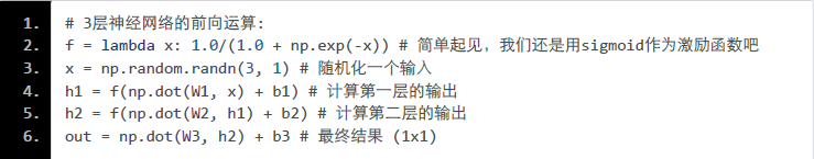
In the code above, W1, W2, W3, b1, b2, and b3 are all parameters of the neural network to be learned. Note that all operations here are vectorized/matrix-ized, so x is no longer a single number but contains the inputs of a batch from the training set, allowing parallel computation to speed up the calculations. Upon careful examination of the code, the last layer does not go through an activation function and directly outputs.

3. Expressive Power of Neural Networks and Size

Once a neural network structure is set up, it contains billions of parameters and functions. We can view it as performing a very complex function mapping on the input to obtain the final result used for spatial partitioning (in classification problems). What influence do our parameters have on this so-called complex mapping?

In fact, a neural network with one hidden layer (2-layer neural network) already possesses the expected capability; as long as the number of neurons in the hidden layer is sufficient, we can always use it (the 2-layer neural network) to approximate any continuous function (i.e., the mapping from input to output). For detailed content, you can refer to Approximation by Superpositions of Sigmoidal Function or Michael Nielsen’s introduction. Our previous blog series on the introductory exploration of neural networks from an elementary mathematics perspective has also mentioned this.

The question is, if a single hidden layer neural network can approximate almost all continuous functions, why do we still use so many layers? Unfortunately, even though mathematically we can approximate almost all functions with a 2-layer neural network, in actual engineering practice, this does not have much effect. Multi-hidden layer neural networks perform much better in engineering than single hidden layer neural networks, even though mathematically their expressive power should be consistent.

However, it should be noted that in general, we find in engineering that 3-layer neural networks perform better than 2-layer neural networks, but if the number of layers continues to increase (4, 5, 6 layers), the improvement in the final results is not as significant. However, in convolutional neural networks, it is different; deep network structures significantly help with accuracy, as images are a type of deep structured data, so deep convolutional neural networks can more accurately express these hierarchical information.

4. Impact of Layer Count and Parameter Settings

A very practical question is, when we encounter a real problem, how do we know how to build a network structure that can best solve this problem? How many layers should be built? How many neurons should each layer have? Let’s understand this intuitively: as we increase the number of layers and the number of neurons in each layer, the capacity of our neural network increases. To put it simply, the spatial expressive capability of the neural network becomes richer. Let’s look at a specific example: suppose we are dealing with a binary classification problem with 2-dimensional input, we train three single-hidden layer neural networks with different numbers of neurons, and their planar expressive capabilities are compared as shown below:

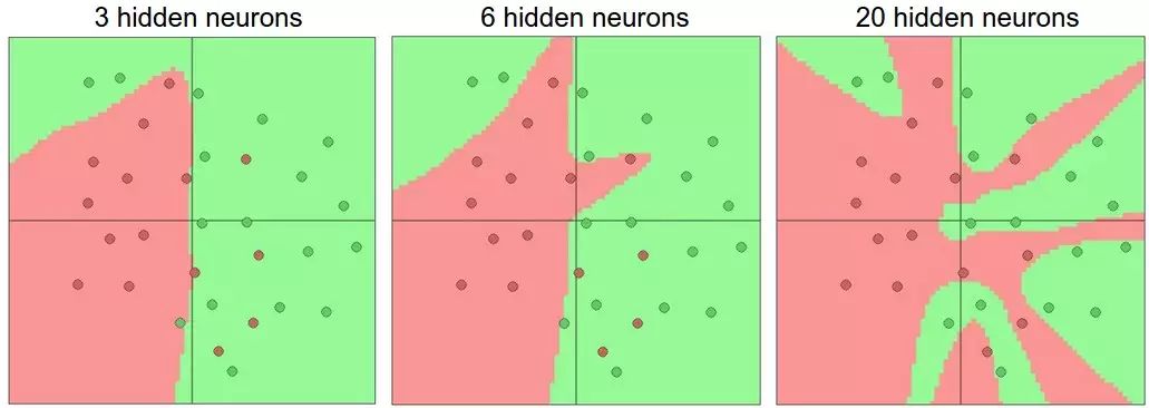
In the above figure, we can see that more neurons allow the neural network to better fit complex spatial functions. However, everything has two sides; the increasing precision of the fit leads to another problem: overfitting too easily!!! If you stubbornly conduct an experiment by placing 20 neurons in the hidden layer, you can achieve 100% separation of the two classes in the above figure, but such a classifier learns and memorizes the distribution of the points on the graph so well that it even learns the noise and outliers, which is a nightmare for our generalization ability on new data.

After our discussion above, you might think that for less complex problems, using fewer layers and neurons might be less prone to overfitting and yield better results. However, this idea is incorrect!!! Never use fewer layers and neurons to alleviate overfitting!!! This will greatly impact the expressive capability of the neural network!!! We have other methods, such as regularization mentioned earlier, to alleviate this issue.

Another reason not to use simple neural networks with fewer layers and neurons is that it is actually more difficult to train suitable parameter results using methods like gradient descent with such simple networks. Yes, you might say that simple neural networks have fewer local minima in their loss functions and should converge better. Yes, that is indeed true; they converge better, but the minima they quickly converge to are usually very poor global minima. In contrast, larger neural networks may have more local minima in their loss functions, but these local minima generally perform better in practice than the poor local minima mentioned above. For non-convex functions, it is challenging to provide 100% accurate proofs of their properties mathematically; if you are interested, you can refer to the paper The Loss Surfaces of Multilayer Networks.

If you are willing to conduct multiple experiments, you will find that training small neural networks results in a significant variation in the minimum value of the loss function. This means that if you are lucky, you may find a relatively suitable set of parameters, but in most cases, the parameters you obtain are just at a not-so-good local minimum. In contrast, larger neural networks do not guarantee convergence to the minimum global minimum, but many local minima have similar performance, meaning you do not need to rely on ‘luck’ to find a near-optimal set of parameters.

Finally, let’s mention regularization; we said we need to use regularization to control overfitting issues. The regularization parameter is , and its size reflects our limitations on the parameter search space. If set small, the parameter’s variability range is large, making overfitting more likely. If set too large, the suppression effect on parameters is too strong, making it difficult to represent class distributions well. The following figure shows the plane segmentation results obtained with different sizes of regularization parameters .

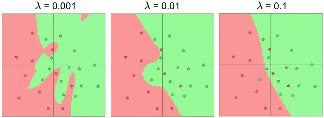
In summary, we often need to use large neural networks with multiple layers and neurons for many practical problems, while using regularization to mitigate overfitting phenomena.

◆ ◆ ◆

Other Reference Materials

• Introduction to Deep Learning with Theano

• Introduction to Neural Networks by Michael Nielsen

• ConvNetJS demo

References and Original Text

http://cs231n.github.io/neural-networks-1/

Regarding Reproduction

If you need to reproduce, please indicate the author and source prominently at the beginning (Reproduced from: Big Data Digest | bigdatadigest) and place a prominent QR code for Big Data Digest at the end of the article. For articles without original identification, please edit according to the reproduction requirements and can be reproduced directly. After reproduction, please send us the reproduction link; for articles with original identification, please send us [Article Name - Public Account Name and ID for Authorization Application]. Unauthorized reproductions and adaptations will be pursued legally. Contact email: [email protected].

◆ ◆ ◆

Big Data Articles on Stanford Deep Learning Courses

Reply “Volunteer” in the backend of Big Data Digest to learn how to join us

Column Editor

Project Management

Content Operations: Wei Zimin

Overall Coordination: Wang Decheng

Recommended previous excellent articles; click the image to read

[Another Heavyweight] Another translation authorization obtained, Stanford CS231N Deep Learning and Computer Vision

Stanford Deep Learning Course Part 7: RNN, GRU, and LSTM

Stanford CS231N Deep Learning and Computer Vision Part 2: Image Classification and KNN