This article is a translated version of the Stanford University CS231N course notes, authorized by Professor Andrej Karpathy of Stanford University. The Big Data Digest work is not allowed to be reproduced without authorization; specific requirements for reproduction can be found at the end of this article.

Translation: Han Xiaoyang & Long Xincheng

Editor’s Note: This article is the second series of the Stanford course articles we bring to readers in the Stanford Deep Learning and Computer Vision Course special series. The content is from the Stanford CS231N series, intended for interested readers to experience and learn.

The video translation of this course is also underway and will be released soon, please stay tuned!

The Big Data Digest will continue to release translations and videos, sharing them for free with all readers.

We welcome more interested volunteers to join us for communication and learning. All translators are volunteers, and if you are capable and willing to share like us, please join us. Reply “Volunteer” in the backend of Big Data Digest to learn more.

The Stanford University CS231N course is a classic tutorial in deep learning and computer vision, highly regarded in the industry. Previously, some friends in China did sporadic translations; to share high-quality content with more readers, Big Data Digest has conducted a systematic and comprehensive translation, and subsequent content will be released gradually.

Due to the inability to edit code in the WeChat backend, we used image insertion to display code; click on the image for a clearer view.

Meanwhile, Big Data Digest has previously obtained authorization for the first series of Stanford courses Stanford University CS224d Course [Machine Learning and Natural Language Processing], which has completed eight sessions. We will continue to push subsequent notes and course videos every Wednesday, please pay attention.

Reply “Stanford” to download related materials for the CS231N series.

Also obtain related materials for another Stanford course CS224d on deep learning and natural language processing.

In addition, for readers interested in further learning and communication, we will organize study exchanges through QQ groups (due to the limit on WeChat group sizes).

Long press the following QR code to jump directly to the QQ group.

Or join the group using the group number 285273721.

◆ ◆ ◆

1. Training

In the previous section, we discussed the static parts of neural networks: including neural network structure, types of neurons, data parts, loss function parts, etc. In this part, we focus on the dynamic aspects, mainly training, emphasizing some points to pay attention to during actual engineering practice, and how to find the most suitable parameters.

1.1 About Gradient Checking

In previous blog posts, we mentioned that we need to compare numerical gradients with gradients obtained from analytical methods. This process is very prone to errors in actual engineering; here are some tips and points to note:

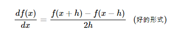
Use the centering formula, which we mentioned before, using the following numerical gradient calculation formula:

instead of

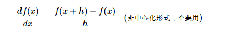
Even though the above form seems to have double the computational load, if you’re interested in expanding the formula in the Taylor series, you’ll find that the error rate of the above formula is about level, while the below formula is O(h), noting that h is a very small number, so the above formula is clearly more accurate.

Use relative error for comparison; this is another point to mention in actual engineering. After obtaining the numerical gradient and analytical gradient , how do we compare the two? The first reaction is to take the difference , right? Or at most, take a square. However, using absolute values is unreliable; if both gradients have absolute values around 1, we might consider a difference of 1e-4 to be very small. But if both gradients are around the magnitude of 1e-4, then this difference is quite large. Therefore, we consider the relative error:

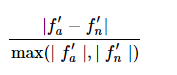
The reason for adding the max term is simple: it makes the overall form simpler and more symmetrical. Another reminder is to avoid cases where both terms in the denominator are 0. For relative error:

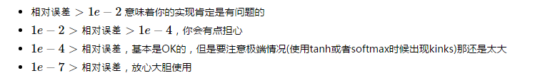Oh, there’s one more thing we need to know: as the number of layers in the neural network increases, the relative error will increase. This means that for a 10-layer neural network, a relative error of around 1e-2 might already be usable.

Use double-precision floating-point numbers. If you compute using single-precision floating-point numbers, your implementation might have no issues, but the relative error could be large. In actual engineering, there have been cases where switching from single to double precision reduced the relative error from 1e-2 to 1e-8.

Be aware of the range of floating-point numbers. A good article is What Every Computer Scientist Should Know About Floating-Point Arithmetic. We must ensure that during calculations, all numbers are within the computable range of floating-point numbers; very small values (like h) can cause computational issues.

Kinks. This refers to situations where numerical gradients and analytical gradients are inconsistent. This can occur when using ReLU or similar neuron units. For very small negative numbers, like x=-1e-6, since x<0, the analytical gradient is absolutely 0. However, for the numerical gradient, if you compute f(x+h) with h>1e-6, it jumps to the positive part, resulting in a discrepancy between the numerical and analytical gradients. This is not an extreme case; for a dataset like CIFAR-10, which has 50,000 samples, each sample corresponds to 9 incorrect categories (contributing 9 loss values to the loss function), leading to 450,000 instances of max(0,x) where many kinks can occur.

However, we can monitor the two terms in max, and if the larger term crosses 0, we need to pay attention.

Be careful in setting the step size h. h should definitely not be too large; everyone knows that. But I’m not saying h should be set very small; actually, setting h very small can also cause problems, as it may lead to precision issues. Interestingly, in practice, sometimes adjusting h from very small to 1e-4 or 1e-6 can suddenly make calculations normal.

Do not let the regularization term overshadow the data term. This problem can occur because the loss function is a sum of the data loss part and the regularization part. Therefore, it is essential to pay special attention to the regularization part. You can imagine that if it overshadows the data part, the main source of the gradient will be from the regularization term, making it impossible to perform normal gradient backpropagation and parameter iterative updates. Therefore, even when checking whether the implementation of the data part is correct, you should first turn off the regularization part (set coefficient λ to 0) before checking.

Be cautious with dropout and other parameters. When checking numerical gradients and analytical gradients, if you do not ‘turn off’ dropout and other parameters, there will definitely be a large difference between the two. However, ‘turning them off’ has the downside of making it impossible to check whether the gradients of these parts are correct. Therefore, a reasonable approach is to randomly initialize x before calculating f(x+h) and f(x−h), and then calculate the analytical gradient.

Regarding checking only a few dimensions. In actual situations, gradients can have millions of parameter dimensions. Therefore, checking each dimension is not very realistic; generally, only a few dimensions are checked, and the assumption is that the other dimensions are also correct. Be careful: ensure that every parameter in these dimensions has been checked and compared.

1.2 Pre-training Checks

Before starting training, we also need to perform some checks to ensure that we do not run for a long time only to find that the training, which incurs a high computational cost, is actually incorrect.

After initialization, take a look at the loss. In fact, after initializing the neural network with very small random numbers, the first calculation of the loss can be a check (of course, remember to set the regularization coefficient to 0). Taking CIFAR-10 as an example, if we use a Softmax classifier, we predict that we should obtain an initial loss value of around 2.302 (because there are 10 categories, the initial probability should be 0.1, and the Softmax loss is -log(correct category probability): -ln(0.1)=2.302).

Add back the regularization term, and then set the regularization coefficient to a small normal value and recalculate the loss; it should be larger than the previous value.

Try to fit a small dataset. The last step, which is also very important, is that before training on a large dataset, we can first train on a small dataset (for example, 20 images) and see if your neural network can achieve 0 loss (of course, this refers to the case where the regularization coefficient is 0), because if the implementation of the neural network is correct, it should be able to overfit this small portion of data without the regularization term.

1.3 Monitoring During Training

Once training begins, we can monitor certain indicators to understand the status of the training. We remember that some parameters are considered finalized, such as learning rate and regularization coefficient.

• Loss/loss changes after each complete iteration

The following chart illustrates how the loss should change after each complete iteration (where a complete iteration means all samples have been passed through, since the batch size setting may vary in stochastic gradient descent, we do not select each mini-batch iteration as a cycle):

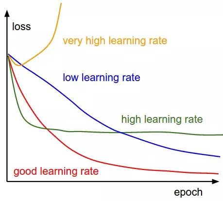
A suitable learning rate can ensure that the loss decreases after each complete training round and can reach a smaller level after some time. With too small a learning rate, the loss decreases very slowly; if set too aggressively with a high learning rate, the initial loss decreases significantly, but after a certain point, it stops decreasing and oscillates without reaching the lowest point. The following chart shows the loss changes during actual training on CIFAR-10:

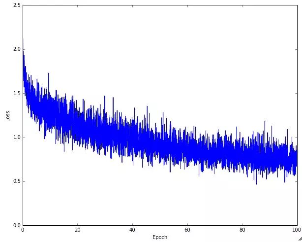
One might notice that the curve in the above chart has some fluctuations and instability, which relates to the batch size set during stochastic gradient descent. When the batch size is very small, there can be significant instability; if the batch size is set larger, it becomes relatively more stable.

• Accuracy on training/validation sets

Next, we need to track the accuracy on the training set and validation set to determine the state of the classifier (how much overfitting is occurring):

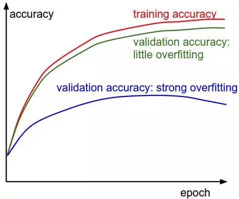
As time progresses, the accuracy on both the training set and validation set should increase. If the accuracy on the training set reaches a certain level and the difference between the two becomes significant, we should be cautious of potential overfitting. If the difference is not large, it indicates that the model is in good condition.

• Weights: Ratio of weight updates

The last quantity to monitor is the ratio of weight update magnitude to the current weight magnitude. Note, this refers to the weight update part, not necessarily the computed gradient (for example, in vanilla SGD, this value is the product of gradient and learning rate). Ideally, we should check this ratio independently for each parameter set. We cannot draw a definite conclusion, but in previous engineering practices, a suitable ratio is around 1e-3. If the ratio you obtain is much smaller than this value, it indicates that the learning rate is set too low; conversely, it is set too high.

• Distribution of activations/gradient values for each layer

If the parameter initialization is incorrect, the entire training process will slow down significantly or even stop. However, we can easily identify this issue. The most apparent data is the variance (fluctuation) of activations and gradients for each layer. For example, if the initialization is incorrect, it is likely that the variance of activations (the input part of the activation function) changes as follows from front to back:

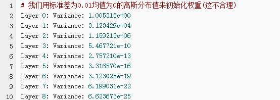
Looking at the above values, one can see that from front to back, the fluctuations in activation values decrease significantly layer by layer, which means that during the backpropagation algorithm, the gradients being calculated will approach 0, thus the parameter updates will almost decay to nothing, making it clearly unreliable. By correctly initializing weights as mentioned in the previous lecture, and observing the variance of activations/gradients layer by layer, it will be found that their variance does not decrease so drastically, remaining at a similar level:

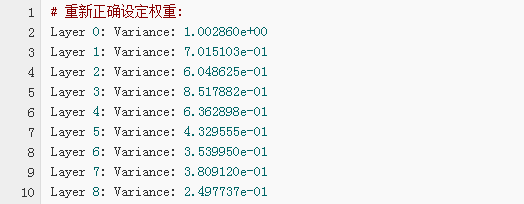Looking at the fluctuations of activations layer by layer, one will find that even in the last layer, the network is still ‘active’, indicating that the gradient values being backpropagated are sufficient, and the neural network is in a positive learning state.

• Visualization of the first layer

Lastly, if the neural network is used for image-related problems, visualizing the features and data from the first layer can help us understand whether training is normal:

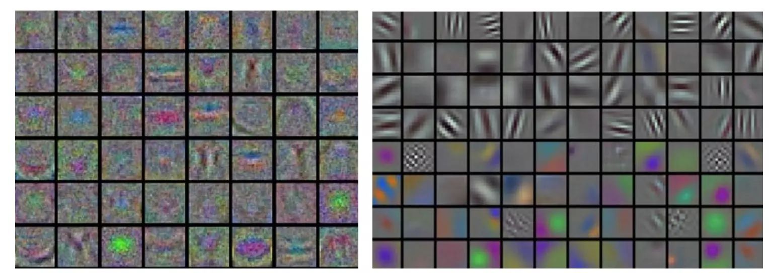
The images on the left and right show a comparison of the first-layer features under normal and abnormal conditions. In the left image, the feature noise is high, and the image is ‘cloudy’, indicating that the training may be in a ‘pathological’ process: perhaps the learning rate is set incorrectly, or the regularization coefficient is too low, or for other reasons, the neural network may not converge. In the right image, the features are smooth and clean, with significant distinction between them, indicating that the training process is relatively normal.

1.4 Notes on Parameter Update

When we are sure that the analytical gradient implementation is correct, we should use it to update the weight parameters in the backpropagation algorithm. Regarding the single parameter update aspect, there are indeed some nuances:

It can be said that the optimization of neural networks is a hot topic in deep learning research. Below are some methods mentioned in the papers by experts, many of which are indeed very effective and commonly used in practice.

1.4.1 Stochastic Gradient Descent and Parameter Updates

Vanilla update

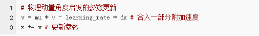
This is the simplest parameter update method. After obtaining the gradient, multiply it by the set learning rate, and subtract this part from the current weights to get the new weight parameters (since the gradient indicates the direction of the maximum increase, subtracting this value will decrease the loss function value). Let x be the weight parameter vector x, and the gradient be dx, then the simplest parameter update everyone knows is:

Of course, learning_rate is a hyperparameter value we set (which remains constant throughout this update method), and mathematically, it can be guaranteed that when the learning rate is sufficiently low, the loss function will not increase after iteration.

Momentum update

This is a small optimization of the above parameter update method, generally speaking, it converges more efficiently (faster) in deeper neural networks. This parameter update method originates from optimization in physics.

Here, v is a value initialized to 0, mu is another hyperparameter we set (the most common value is 0.9, which relates to the coefficient of friction), a rough understanding is that stochastic gradient descent can be seen as a process of going down a mountain, and this method adds a certain frictional resistance during the descent, consuming a small portion of the energy of the power system, allowing it to stop at the bottom more efficiently instead of oscillating continuously. By the way, we can also use cross-validation to select the most suitable mu value, generally selecting the most suitable from [0.5, 0.9, 0.95, 0.99].

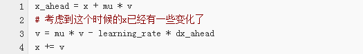
Nesterov Momentum

This is a different version of the momentum update, which has recently become very popular. It is said that this parameter update method has a better theoretical basis in convex functions and convex optimization, and its convergence effect in practice is slightly better than that of momentum update.

The deeper principles behind it, I find a bit challenging… Interested students can refer to the following two materials:

• Yoshua Bengio’s Advances in optimizing Recurrent Networks section 3.5

• Ilya Sutskever’s thesis section 7.2

Its concept corresponds to the following code:

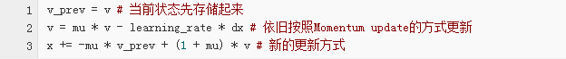
A more practical version in engineering is:

1.4.2 Decaying Learning Rate

In the actual training process, it is often necessary to gradually decay the learning rate as training progresses. Returning to the mountain scenario, when first descending, we may be far from the lowest point, so taking larger steps is fine; however, as we approach the foot of the mountain, if we continue to take aggressive steps, we may accidentally overshoot. Therefore, it is better to gradually slow down the pace as we descend. However, this ‘timing’ needs to be carefully controlled; if the decay is too slow, oscillations may still occur at the lowest point; if it decays too quickly, the entire system’s ‘momentum’ decreases too quickly, and it will soon stop descending. Below are some common learning rate decay methods:

• Step decay: This is a very common decay pattern where the learning rate decreases after every complete training cycle (after all images have been processed). For example, a common decay rate might be to decrease by 10% every 20 complete training cycles. However, the most suitable value does vary by problem. If during training, you find a high error rate on the cross-validation set that does not decrease, you might consider adjusting (decaying) the learning rate.

• Exponential decay: The mathematical form is α=α0e−kt, where α0 and k are hyperparameters that need to be set, and t is the number of iterations.

• 1/t decay: The decay pattern has the mathematical form α=α0/(1+kt), where α0 and k are hyperparameters that need to be set, and t is the number of iterations.

In practice, many people prefer using step decay because it involves fewer hyperparameters, is simpler to compute, and has slightly better interpretability.

1.4.3 Second Order Iterative Methods

Another well-known optimization method in optimization problems is Newton’s method, which updates parameters as follows: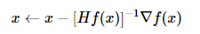

Here, Hf(x) is the Hessian matrix, which is the second-order partial derivative of the function. And is a gradient vector similar to what is seen in gradient descent. The intuitive understanding is that the Hessian matrix describes the curvature of the loss function, allowing us to update parameters more efficiently and approach the lowest point: multiplying by the Hessian matrix during parameter iteration allows for more aggressive parameter updates in regions of flatter curvature, while in steep regions, the steps will slow down. Thus, compared to first-order updating algorithms, it has significant advantages.

However, the awkward part is that in actual deep learning processes, directly using second-order iterative methods is not very practical. The reason is that directly computing the Hessian matrix is a very resource-intensive process. For example, a neural network with one million parameters has a Hessian matrix dimension of [1000000*1000000], which would take up 3725G of memory. Of course, we have algorithms like L-BFGS that approximate the Hessian matrix to solve the memory problem. However, L-BFGS generally computes on the entire dataset, unlike our mini-batch SGD that iterates on small batches. Many researchers are currently working on this problem, trying to enable L-BFGS to stably update in a mini-batch manner. But for now, large-scale deep learning rarely uses L-BFGS or similar second-order iterative methods; rather, simple algorithms like stochastic gradient descent are widely used.

Interested students can refer to the following literature:

• On Optimization Methods for Deep Learning: A 2011 paper comparing stochastic gradient descent and L-BFGS.

• Large Scale Distributed Deep Networks: A paper from the Google Brain team comparing the differences between stochastic gradient descent and L-BFGS in large-scale distributed optimization.

• The SFO algorithm attempts to combine the advantages of stochastic gradient descent and L-BFGS.

1.4.4 Per-Parameter Learning Rate Updates

So far, the learning rate update methods you have seen have all used the same learning rate globally. Adjusting the learning rate is a time-consuming and error-prone task; thus, there has been a desire for a self-updating learning rate method that can even be refined to per-parameter updates. There are indeed some methods like this now, most of which require additional hyperparameter settings, but the advantage is that under most hyperparameter settings, they perform better than using fixed learning rates. Below are some common adaptive methods (please forgive the blogger’s limited background, I cannot delve into the mathematical details):

Adagrad is an adaptive learning rate algorithm proposed by Duchi et al. in the paper Adaptive Subgradient Methods for Online Learning and Stochastic Optimization. A simple code implementation is as follows:

In this case, the variable cache has the same dimensions as the gradient, and we continuously accumulate the square of the gradient with this variable. This value is then used for normalization in the parameter update step. The benefit of this method is that for weights with high gradients, their effective learning rates are reduced; while for weights with small gradients, the learning rate is increased during the iteration. The square root step is very important; not taking the square root leads to far inferior results. The smoothing parameter 1e-8 avoids division by zero situations.

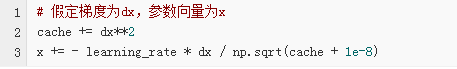
RMSprop is a very effective adaptive learning rate update method, although it seems not to have been publicly released. Interestingly, people using this method all cite Geoff Hinton’s Coursera course lecture 6, page 29. The RMSProp method makes a simple optimization to the Adagrad algorithm to reduce its iteration intensity, roughly illustrated in the following code:

Here, decay_rate is a manually set hyperparameter, and we usually choose it from [0.9, 0.99, 0.999]. It is particularly important to note that the accumulation part of x+= is exactly the same as in Adagrad, but the cache itself is iteratively changing.

Other methods include:

• Adadelta proposed by Matthew Zeiler.

• Adam: A Method for Stochastic Optimization.

• Unit Tests for Stochastic Optimization.

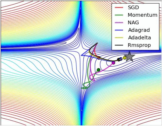
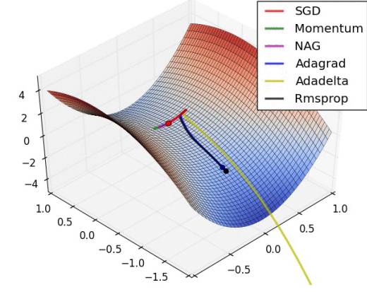
The following chart illustrates the optimization of the loss function under various parameter update methods:

1.5 Setting and Optimizing Hyperparameters

During the training process of neural networks, we inevitably deal with many hyperparameters that we need to set manually, including:

• Initial learning rate.

• Learning rate decay degree.

• Regularization coefficient/strength (including l2 regularization strength, dropout ratio).

For large, deep neural networks, we need a lot of time for training. Therefore, spending some time on hyperparameter search beforehand to determine the best settings is very necessary. The most direct way is to design a process during the framework implementation that continuously changes hyperparameters for optimization and records the validation set status and effects for each complete training iteration under each hyperparameter.

In actual engineering, when determining these hyperparameters in neural networks, we generally do not use k-fold cross-validation; instead, a fixed cross-validation set is sufficient.

Generally, attempts and searches for hyperparameters are conducted in the log domain. For example, a typical learning rate search sequence is learning_rate = 10 ** uniform(-6, 1). We first generate a uniformly distributed sequence and then perform exponentiation with base 10; we actually apply the same strategy in the regularization coefficient. For instance, a common search sequence is [0.5, 0.9, 0.95, 0.99]. Additionally, it is essential to note that if the best hyperparameter results obtained from cross-validation are at the edge of the distribution, we should be particularly cautious; the range taken for uniform distribution may itself be unreasonable, and expanding this search range may yield better parameters.

1.6 Model Fusion and Optimization

In practical engineering, an effective way to improve the final performance of neural networks is to train multiple independent models and select the mode of the results during the prediction phase. Model fusion can alleviate overfitting to some extent and help improve the final results. We have several ways to obtain different independent models for the same problem:

• Using different initialization parameters. First, determine the best hyperparameters using cross-validation, and then select different initial values for training, resulting in models with some differences.

• Selecting models that rank high in cross-validation. When determining hyperparameters using cross-validation, select the top hyperparameters, and train and model them separately.

• Selecting models at different time points during training. Training neural networks is indeed a time-consuming task; therefore, some people take models from different time points after the model reaches a certain accuracy. However, it is quite evident that the differences between such models are relatively small, and the benefit is that one-time training can yield the benefits of model fusion.

Another commonly used effective method to improve model performance is to retain several intermediate model weights and the final model weights during the later stages of training, average them, and then test the results on the cross-validation set. This usually yields results that are one or two percentage points higher than those of the directly trained model. The intuitive understanding is that for a bowl-shaped structure, many times our weights oscillate near the lowest point but cannot truly reach it; averaging two positions near the lowest point has a higher probability of landing closer to the lowest point.

◆ ◆ ◆

2. Summary

• Test your gradient calculations with a portion of the data, paying attention to the mentioned points.

• Check whether your initial weights are reasonable and whether you can achieve 100% accuracy in a system without regularization terms.

• During training, record the results of the loss function, as well as the accuracy on the training set and cross-validation set.

• The most common weight update method is SGD+Momentum; try the RMSProp adaptive learning rate update algorithm.

• Use different methods to decay the learning rate over time.

• Use cross-validation, etc., to search for and find the most suitable hyperparameters.

• Remember to also perform model fusion work, which can be helpful for results.

Regarding Reproduction

If you need to reproduce, please prominently indicate the author and source at the beginning of the article (reproduced from: Big Data Digest | bigdatadigest), and place a prominent QR code for Big Data Digest at the end of the article. Articles without original identification can be edited according to reproduction requirements and reproduced directly; please send us the reproduction link after reproduction; for articles with original identification, please send [Article Name - Pending Authorized Public Account Name and ID] to us to apply for whitelist authorization. Unauthorized reproduction and adaptation will be pursued legally. Contact email: [email protected].


◆ ◆ ◆

Big Data Articles on Stanford Deep Learning Courses

Reply “Volunteer” in the Big Data Digest backend to learn how to join us.

Column Chief Editor

Project Management

Content Operations: Wei Zimin

Coordination: Wang Decheng

Previous Excellent Articles Recommended, click the images to read.

Stanford CS231N Deep Learning and Computer Vision Episode 7: Neural Network Data Preprocessing, Regularization, and Loss Function

Stanford 224d Deep Learning Course Episode 7: RNN, GRU, and LSTM

Stanford CS231N Deep Learning and Computer Vision Episode 6: Neural Network Structure and Neuron Activation Functions