This article is a translated note of the Stanford University CS231N course, authorized for translation and publication by Professor Andrej Karpathy of Stanford University. This is a work from Big Data Digest, unauthorized reproduction is prohibited; specific requirements for reproduction can be found at the end of the article.

Translation: Han Xiaoyang & Long Xincheng

Editor’s Note: This article is the second installment of the Stanford Deep Learning and Computer Vision course series that we bring to our readers. The content is from the Stanford CS231N series, intended for interested readers to experience and learn.

The video translation for this course is also underway and will be released soon, so please stay tuned!

Big Data Digest will continue to publish translations and videos, sharing them for free with all readers.

We welcome more interested volunteers to join us for mutual exchange and learning. All translators are volunteers; if you, like us, are capable and willing to share, please join us. Reply “Volunteer” to the Big Data Digest backend for more information.

The Stanford University CS231N course is a classic tutorial on deep learning and computer vision, highly regarded in the industry. Previously, some friends in China did some sporadic translations. To share high-quality content with more readers, Big Data Digest has conducted a systematic and comprehensive translation, with subsequent content to be released gradually.

Since the code editing in WeChat’s backend cannot be realized, we have used images to display the code. Click on the image to view a clearer version.

Additionally, Big Data Digest has previously obtained authorization for the first series of the Stanford course Stanford University CS224d Course [Machine Learning and Natural Language Processing], which has completed seven lessons. We will continue to push subsequent content and course videos every Wednesday, so please pay attention.

Moreover, for readers interested in further learning and communication, we will organize study exchanges via QQ groups (due to the limitation of WeChat group size).

Long press the QR code below to jump directly to the QQ group

Or join the group using the group number 564538990

◆ ◆ ◆

Introduction

This is something that people do naturally every day, so ordinary that most of the time we are unaware that we are completing such tasks. When you wake up in the morning and wash up, you need to see which one among the many items on the washstand is your cup, and which is your toothbrush; during breakfast, you need to distinguish between food and dishes…

Abstractly, for an input image, we need to determine which of the given labels/categories it belongs to. This seems like a simple problem, yet it has been a core issue in computer vision for many years, with many application scenarios. Its importance is also reflected in the fact that other computer vision problems (such as object localization and recognition, image segmentation, etc.) can be completed based on it.

◆ ◆ ◆

1. Image Classification

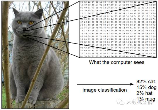
The computer receives an image (as shown below), and then needs to provide the probabilities corresponding to the four categories {cat, dog, hat, cup}. Humans are incredibly capable beings; we can tell at a glance that it is a cat. However, for computers, they cannot ‘see’ the entire image like humans. For them, it is a 3-dimensional matrix containing 248*400 pixels, with each pixel having values for red, green, and blue (RGB) color channels, each value ranging from 0 (black) to 255 (white). The computer needs to determine that this is a ‘cat’ based on these 248*400*3=297600 values.

1.1 The Challenges of Image Recognition

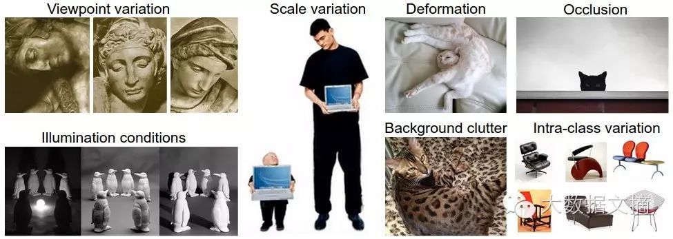
Image recognition seems very straightforward. However, it contains many challenges. Humans have evolved over hundreds of millions of years to acquire such a powerful brain and have precise visual understanding of various objects. Overall, when we want to ‘teach’ a computer to recognize a class of images, we encounter the following difficulties:

Different angles; each object may look completely different when rotated or viewed from the side.
Inconsistent sizes; images of the same content can be large or small.
Deformation; many objects may have special placements and shapes under specific circumstances.
Interference/illusion from light and shadow.
Background interference.
Differences within the same category (for example, chairs can be armchairs/bar stools/dining chairs/recliners…)

1.2 Approaches to Recognition

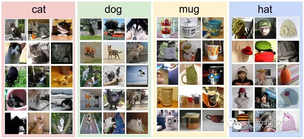
First, it’s easy to see that this algorithm is not like ‘sorting an array’ or ‘finding the shortest path in a directed graph’; we cannot predefine a process and rules to solve it. Defining what a ‘cat’ is, is already a challenging task, let alone defining a fixed representation of a cat in an image. Therefore, we hope to use machine learning and a ‘Data-driven approach’ to make some attempts. In simple terms, for each category, we find a certain amount of image data to ‘feed’ the computer so that it can ‘learn and summarize’ the characteristics of each category of images. This process is akin to how a child learns about new things. The images we ‘feed’ the computer for learning are like the following images of cats/dogs/cups/hats:

1.3 The Process/Pipeline for Machine Learning to Solve Image Classification

The overall process is consistent with ordinary machine learning, simply put, it consists of the following three steps:

Input: Our given N images of K categories, as the training set for the computer to learn.
Learning: Let the computer ‘observe’ and ‘learn’ image by image.
Evaluation: Just like how we take exams to test what we learned in school, we also need to test how well the computer has learned. Thus, we provide some images with unknown categories for the computer to classify and then compare with the known correct answers.

2. Nearest Neighbor Classifier

◆ ◆ ◆

2. Nearest Neighbor Classification Method

Let’s start with a simple method, the nearest neighbor classifier. However, it should be noted that it has no relation to convolutional neural networks in deep learning; we are just progressing from basic to advanced step by step. The nearest neighbor is a relatively simple and basic implementation of image recognition.

2.1 CIFAR-10

CIFAR-10 is a very commonly used image classification dataset. The dataset contains 60,000 small images of size 32*32 pixels, with each image having a category label (a total of 10 categories), divided into a training set of 50,000 images and a test set of 10,000 images. Below are some example images:

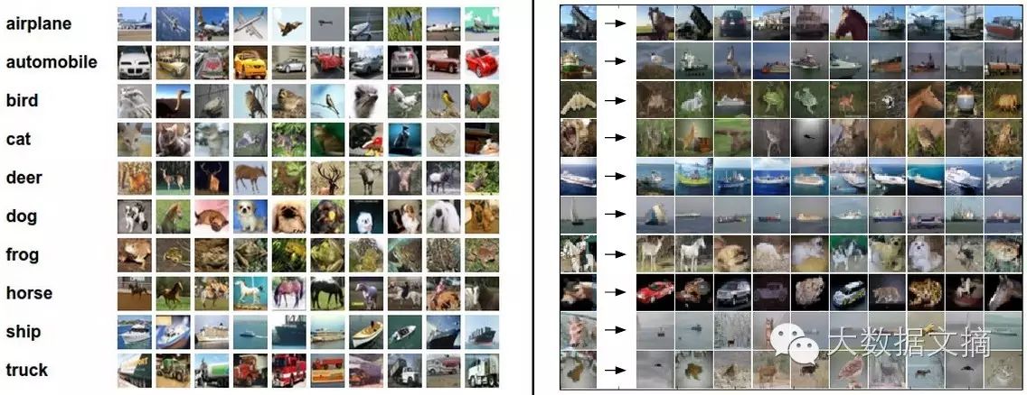
In the image above, the left shows the ten categories and some corresponding example images, while the right shows the ten nearest images calculated based on pixel distance when given a specific image.

2.2 Simple Image Category Determination Based on Nearest Neighbors

Now, suppose we use the CIFAR-10 dataset as the training set to determine which category an unknown image belongs to. A very intuitive idea is that since we have the values of each pixel, we can calculate the distance to the images in the training set based on these values, find the nearest image, and use its category as the determined category.

Yes, this idea is direct; this is the ‘nearest neighbor’ concept. Just a side note, this direct method does not perform particularly well in image recognition. For instance, the images found based on this idea only have 3 images with the correct nearest category.

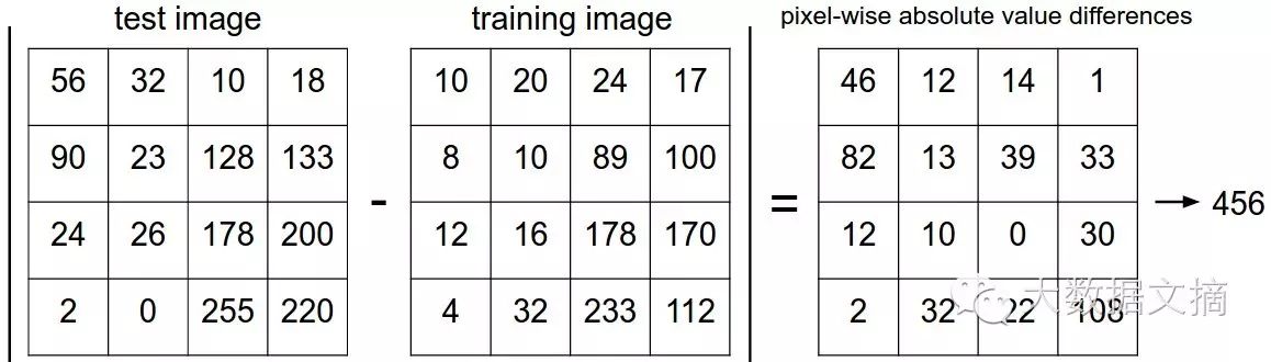
Even so, as the most basic method, it is still essential to master. Let’s implement it simply. We need a criterion for evaluating image distance, such as the simplest method, which is to compare the L1 distance (also known as Manhattan distance/cityblock distance) between two image pixel vectors, as shown in the formula below:

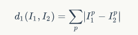
This essentially calculates the difference between all pixel points and sums them up, as intuitively illustrated below:

First, let’s read the dataset into memory:

#! /usr/bin/env python
#coding=utf-8
import os
import sys
import numpy as np
def load_CIFAR_batch(filename):
 """
 The CIFAR-10 dataset is stored in batches; this function loads a single batch.
 @param filename: CIFAR filename
 @return: X, Y: data and labels in the CIFAR batch
 """
 with open(filename,'r')as f:
 datadict=pickle.load(f)
 X=datadict['data']
 Y=datadict['labels']
 X=X.reshape(10000,3,32,32).transpose(0,2,3,1).astype("float")
 Y=np.array(Y)
 return X, Y
def load_CIFAR10(ROOT):
 """
 Load the entire CIFAR-10 dataset
 @param ROOT: root directory name
 @return: X_train, Y_train: training data and labels
 X_test, Y_test: test data and labels
 """
 xs=[]
 ys=[]
 for b in range(1,6):
 f=os.path.join(ROOT,"data_batch_%d"%(b,))
 X, Y=load_CIFAR_batch(f)
 xs.append(X)
 ys.append(Y)
 X_train=np.concatenate(xs)
 Y_train=np.concatenate(ys)
 del X, Y
 X_test, Y_test=load_CIFAR_batch(os.path.join(ROOT,"test_batch"))
 return X_train, Y_train, X_test, Y_test
# Load training and testing datasets
X_train, Y_train, X_test, Y_test = load_CIFAR10('data/cifar10/')
# Flatten the 32*32*3 multidimensional array
Xtr_rows= X_train.reshape(X_train.shape[0],32*32*3)# Xtr_rows : 50000 x 3072
Xte_rows= X_test.reshape(X_test.shape[0],32*32*3)# Xte_rows : 10000 x 3072

Next, let’s implement the nearest neighbor approach:

classNearestNeighbor:
 def __init__(self):
 pass
 def train(self, X, y):
 """ 
 The training here is actually just reading all the existing images into memory -_-||
 """
 # The nearest neighbor classifier simply remembers all the training data
 self.Xtr= X
 self.ytr = y
 def predict(self, X):
 """ 
 The prediction process is actually scanning all the images in the training set, calculating distances, and taking the label of the image with the smallest distance.
 """
 num_test = X.shape[0]
 # Ensure dimensions match
 Ypred= np.zeros(num_test, dtype = self.ytr.dtype)
 # Scan through the training set
 for i in xrange(num_test):
 # Calculate L1 distance and find the nearest image
 distances = np.sum(np.abs(self.Xtr- X[i,:]), axis =1)
 min_index = np.argmin(distances)# Get the index of the nearest image
 Ypred[i]= self.ytr[min_index]# Record the label
 returnYpred
nn =NearestNeighbor()# Initialize a nearest neighbor object
nn.train(Xtr_rows, Y_train)# Training... actually just reading the training set
Yte_predict= nn.predict(Xte_rows)# Prediction
# Compare with the standard answer and calculate the accuracy
print'accuracy: %f'%( np.mean(Yte_predict== Y_test))

The accuracy obtained from the nearest neighbor method on CIFAR is 38.6%. We know there are 10 categories, and if we guess randomly, the accuracy would be about 1/10=10%. Therefore, it still has some recognition effect, but clearly, it is far lower than the human recognition accuracy (94%), making it not very practical.

2.3 About Distance Criteria for Nearest Neighbors

The distance criterion we used here is the L1 distance; in fact, apart from the L1 distance, we have many other distance criteria.

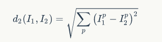
For example, the calculation criterion for L2 distance (the well-known Euclidean distance) is as follows:

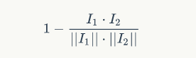
For example, the calculation criterion for cosine distance is as follows:

More distance criteria can be found on the scipy related calculation page.

◆ ◆ ◆

3. K-Nearest Neighbor Classifier

This is an adjustment to the nearest neighbor concept. When we use the nearest neighbor classifier for classification and scan the CIFAR training set, we sometimes find that the nearest image may not necessarily belong to the same category as the current image, but among the nearest ones, there may be many that are of the same category. So it naturally occurs to us to extend the nearest neighbor to the nearest N points and then count the class distribution of these points, taking the most frequent category as our own category.

Yes, this is the idea of KNN.

KNN is actually a very commonly used classification algorithm. However, there is a problem: what should our K value be? In other words, how many neighbors should we find to vote for a reliable classification?

3.1 Cross-Validation and Parameter Selection

In the current scenario, if we decide to use KNN for image category recognition, we find that some parameters will definitely affect the final recognition results, such as:

Choice of distance (L1, L2, cosine, etc.)
Value of the number of neighbors K.

Each set of parameters can produce a new model, so this can be seen as a model selection problem. The most commonly used method for model selection is to experiment on the cross-validation set.

Since the total amount of data is limited, if we perform model parameter selection on the test data and then use it for effect evaluation, it is clearly not very reasonable (because our model parameters are likely to overfit on the test data, and cannot evaluate the results fairly). Therefore, we usually divide the training data into two parts, a large part for training and another part as the so-called cross-validation dataset for model parameter selection. For instance, if we have 50,000 training images, we can split them into 49,000 for training and 1,000 for cross-validation.

# Assuming we already have Xtr_rows, Ytr, Xte_rows, Yte, where Xtr_rows is a 50000*3072 matrix
Xval_rows=Xtr_rows[:1000,:]# Construct 1000 cross-validation set
Yval=Ytr[:1000]
Xtr_rows=Xtr_rows[1000:,:]# Keep 49000 training set
Ytr=Ytr[1000:]
# Set some k values for experimentation
validation_accuracies =[]
for k in[1,3,5,7,10,20,50,100]:
 # Initialize object
 nn =NearestNeighbor()
 nn.train(Xtr_rows,Ytr)
 # Modify the predict function to accept k as a parameter
 Yval_predict= nn.predict(Xval_rows, k = k)
 acc = np.mean(Yval_predict==Yval)
 print'accuracy: %f'%(acc,)
 # Output results
 validation_accuracies.append((k, acc))

Here, I would like to mention a concept that you will see in many places, called k-fold cross-validation, which means dividing the original data into k parts, using k-1 parts as training data while the remaining 1 part serves as cross-validation data (thus we actually obtain k accuracy values for k-fold cross-validation). Below is an example of 5-fold cross-validation:

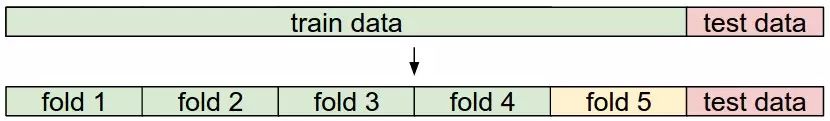
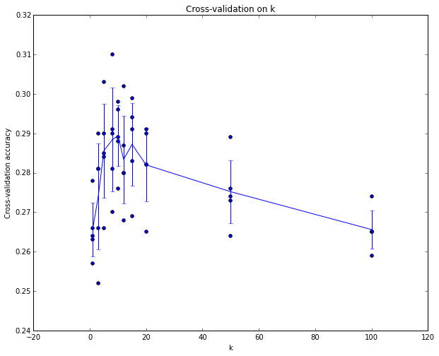
The following is the accuracy curve obtained when using 5-fold cross-validation with different k values (to supplement, since this is 5-fold cross-validation, there are 5 values for each k value, and we take the average as the accuracy at that time). It can be seen that the best accuracy is around k=7.

3.2 Advantages and Disadvantages of Nearest Neighbor Methods

The advantages of K-Nearest Neighbors are clear to everyone; the approach is very simple and clear, and it requires no training at all… However, because of this, the final prediction process is very time-consuming, as it requires comparing with all images in the training set.

In practical applications, we are more concerned about the time consumed for prediction. If an image recognition app takes half an hour or an hour to return results, you would definitely uninstall it immediately. We are not so concerned about the training duration; it’s okay if training takes a little longer, as long as the recognition speed is fast and effective during application, that would be great. The deep neural networks mentioned later are like this; training is a relatively time-consuming process for deep neural networks when solving image problems, but the recognition process is very fast.

Additionally, it must be mentioned that optimizing the computation time for K-Nearest Neighbors remains a very hot topic to this day. The Approximate Nearest Neighbor (ANN) algorithm sacrifices a small portion of accuracy to significantly increase speed and can quickly find approximate K nearest neighbors. Many libraries, such as FLANN, already exist for this purpose.

Finally, let’s illustrate with an image that using pixel-level distances to implement image category recognition has its shortcomings. We use a technique called t-SNE to lay out all images in CIFAR-10 across two dimensions; images that are closer together indicate that their pixel-level distances are closer. However, at a glance, we find that the nearest images are not necessarily of the same category.

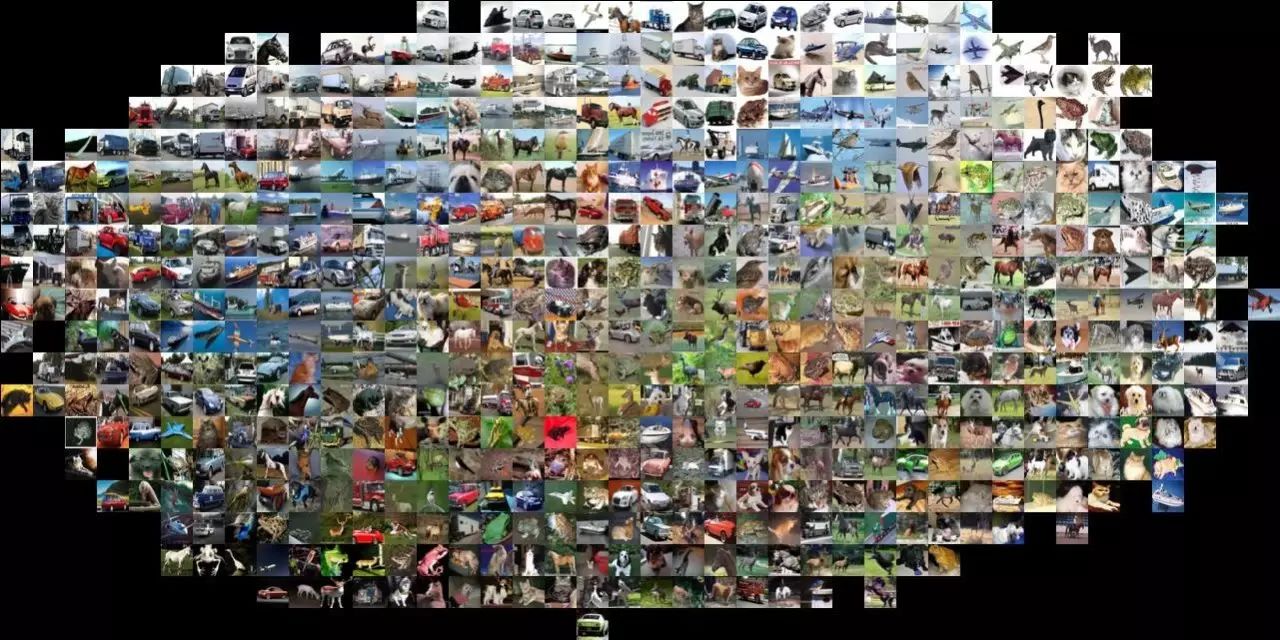
Upon observation, you will find that images that are close in pixel-level tend to share significant commonality in color distribution across the entire image, yet in terms of image content, sometimes we can only helplessly smile, as there are indeed many different objects with similar color distributions.

Reference materials and original text:cs231n Image Classification and KNN

About Reproduction

If you need to reproduce, please indicate the author and source prominently at the beginning (transferred from: Big Data Digest | bigdatadigest), and place a prominent QR code for Big Data Digest at the end of the article. Articles without original markings can be edited according to reproduction requirements and directly reproduced; after reproduction, please send us the reproduction link; for articles with original markings, please send [Article Name - Pending Authorized Public Account Name and ID] to apply for whitelist authorization. Unauthorized reproduction and adaptation will be pursued legally. Contact email: [email protected].

◆ ◆ ◆

Big Data Articles Stanford Deep Learning Course

Reply “Volunteer” to the Big Data Digest backend to learn how to join us

Column Editor

Project Management

Content Operation: Wei Zimin

Coordination: Wang Decheng

Previous Wonderful Articles Recommended, click the image to read

Overview of Machine Learning Algorithms (with Python and R code)

Stanford CS231N Deep Learning and Computer Vision: Image Classification and KNN

Can’t Become a Data Scientist? No Problem, You Can Still Have Data Thinking

Stanford CS231N Deep Learning and Computer Vision: Image Classification and KNN

[Another Heavyweight] Authorization for Translation Again Obtained, Stanford CS231N Deep Learning and Computer Vision

Stanford CS231N Deep Learning and Computer Vision: Image Classification and KNN

Stanford CS231N Deep Learning and Computer Vision: Image Classification and KNN

◆ ◆ ◆

Introduction

◆ ◆ ◆

1. Image Classification

1.2 Approaches to Recognition

2. Nearest Neighbor Classifier

◆ ◆ ◆

2. Nearest Neighbor Classification Method

2.1 CIFAR-10

2.2 Simple Image Category Determination Based on Nearest Neighbors

2.3 About Distance Criteria for Nearest Neighbors

◆ ◆ ◆

3. K-Nearest Neighbor Classifier

3.1 Cross-Validation and Parameter Selection

3.2 Advantages and Disadvantages of Nearest Neighbor Methods

Stanford Deep Learning Course Episode Seven: RNN, GRU, and LSTM

Leave a Comment Cancel reply