
Source | Zhihu
Address | https://zhuanlan.zhihu.com/p/31096913
Author | Datartisan
Editor | Machine Learning Algorithms and Natural Language Processing Public Account
This article is for academic sharing only. If there is any infringement, please contact the background for deletion.
This article will explore efficient deep learning methods using the LSTM neural network approach in TensorFlow.
Sentiment Analysis Based on LSTM Method
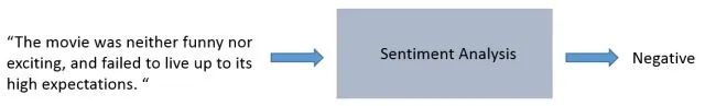
In this note, we will study how to apply deep learning techniques to sentiment analysis tasks. Sentiment analysis can be understood as selecting paragraphs, documents, or any fragment of natural language, then determining whether the text has a positive, negative, or neutral emotional tone.
This note will cover several topics, such as word vectors, time-recurrent neural networks, and long short-term memory. After gaining a good understanding of these terms, we will provide detailed code examples and a complete TensorFlow sentiment classifier at the end.
Before diving into the specifics, let’s first discuss why deep learning is suitable for natural language processing (NLP) tasks.
Applications of Deep Learning in Natural Language Processing
Natural language processing is about creating systems that process or “understand” language to perform certain tasks. These tasks may include:
-
Question answering – the main work of technologies like Siri, Alexa, and Cortana
-
Sentiment analysis – determining the emotional tone behind a segment of text
-
Image to text mapping – generating descriptive text for input images
-
Machine translation – translating a segment of text into another language
-
Speech recognition – computers recognizing spoken language
In the era of deep learning, NLP is a thriving field that has made many different advances. However, there is still a lot of feature engineering work required for all the achievements in the tasks mentioned above, necessitating extensive domain expertise. Practitioners need to master terms like phonemes and morphemes, often spending four years obtaining degrees specifically studying this field. In recent years, deep learning has made remarkable progress, significantly reducing the demand for rich domain knowledge. With a lower barrier to entry, applications of NLP have become one of the largest areas of deep learning research.
Word Vectors
To understand how to apply deep learning, one can think of all the different forms of data that can be applied in machine learning or deep learning models. Convolutional neural networks use pixel value vectors, logistic linear regression uses quantized features, and reinforcement learning models use feedback signals. The commonality is that they all require scalar or scalar matrices as input. When you think about NLP tasks, such data pipelines may come to mind.
This channel has a problem. We cannot perform common operations like dot products or backpropagation on a single string. We need to convert each word in the sentence into a vector rather than just inputting the string.
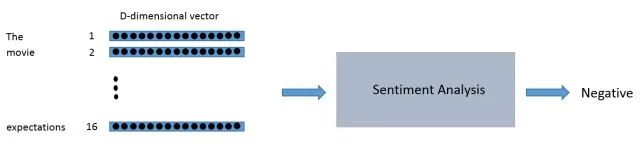
You can think of the input to the sentiment analysis module as a 16 x D dimensional matrix.
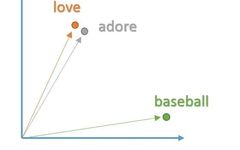
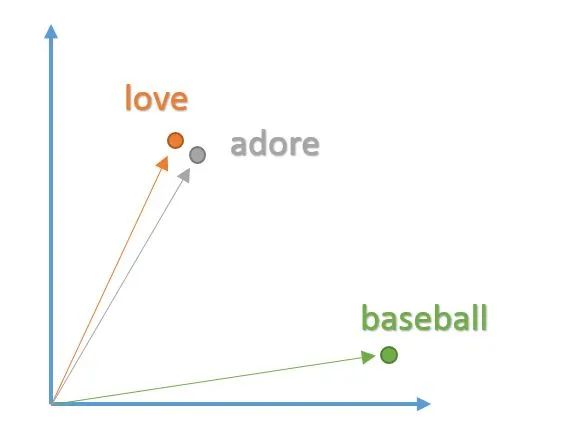
We want to create these vectors in a way that conveniently represents the words and their context, meaning, and semantics. For example, we want the vectors for “love” and “worship” to reside in relatively the same area of vector space, as they have similar definitions and are used in similar contexts. A word’s vector representation is also known as a word embedding.
Word2Vec
To create these word embeddings, we will use a model commonly referred to as “Word2Vec”. The model creates word vectors by looking at the context in which words appear in sentences while ignoring details. Words with similar contexts will be placed close together in vector space. In natural language, the context of a word can be very important when trying to determine its meaning. As we saw earlier with “worship” and “love”,
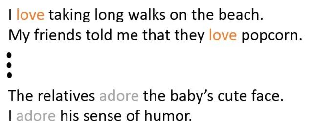
From the context of the sentence, it can be seen that these two words are often used in sentences with positive connotations, typically before nouns or noun phrases. This indicates that both words have something in common and may be synonyms. Considering the grammatical structure of the sentence is also important for context. Most sentences will follow traditional patterns where verbs follow nouns, adjectives precede nouns, and so on. Therefore, the model is more likely to associate nouns with other nouns. The model takes a large dataset of sentences (e.g., English Wikipedia) and outputs vectors for each different word in the corpus. The output of the Word2Vec model is called the embedding matrix.

This embedding matrix will contain vectors for each different word in the training corpus. Traditionally, the embedding matrix can contain over 3 million word vectors.
The Word2Vec model is trained by sliding a fixed-size window over each sentence in the dataset and trying to predict the center word of the window based on the other words given. Using a loss function and optimizer, the model generates vectors for each different word. The specific details of this training process can be a bit complex, so we will skip the details for now, but it is important to note that any deep learning method for NLP tasks is likely to have word vectors as input.
For more information on the theory behind Word2Vec and how to create your own embedding matrix, please check out TensorFlow’s tutorial.
Recurrent Neural Networks (RNNs)
Now that we have our word vectors as input, let’s first look at the actual network architecture we will build. The uniqueness of NLP data is that it has a temporal aspect. The meaning of each word in a sentence largely depends on what has occurred in the past or what will occur in the future.
You will soon see that the structure of recurrent neural networks is a bit different from traditional feedforward neural networks. Feedforward neural networks consist of input nodes, hidden units, and output nodes.
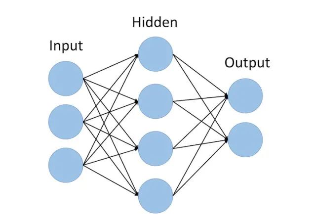
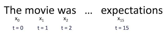
The main difference between feedforward neural networks and recurrent neural networks is the temporal aspect of the latter. In an RNN, each word in the input sequence is associated with a specific time step. In fact, the number of time steps will equal the maximum sequence length.
A new component called the hidden state vector (ht) is also associated with each time step. At a high level, this vector is designed to encapsulate and summarize all the information seen in previous time steps. Just as xt encapsulates all the information of a specific word, ht is a vector that summarizes all the information from previous time steps.
The hidden state is a function of the current word vector and the previous time step’s hidden state. σ represents the sum of the two and is fed into an activation function (usually sigmoid or tanh).
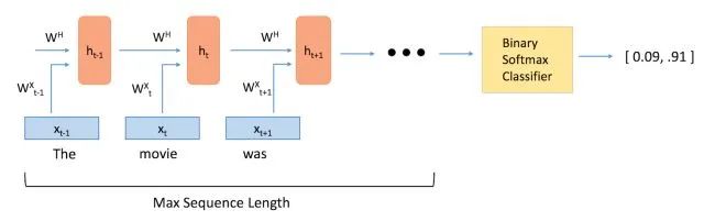
The two W terms in the above equation represent weight matrices. If you take a close look at the superscripts, you will see there is a weight matrix WX that will be multiplied with our input, and there is a recurrent weight matrix WH that will be multiplied with the hidden state from the previous time step. WH remains constant across all time steps, while the weight matrix WX is different for each input.
The size of these weight matrices will affect the variables impacted by the current hidden state or the previous hidden state. As an exercise, refer to the equation above and think about how changes in the values of WX or WH would affect ht.
Let’s look at a simple example: if WH is large and WX is small, I know that ht is greatly influenced by ht-1 and less influenced by xt. In other words, the word corresponding to the current hidden state vector is globally irrelevant in the sentence, so it would be almost the same as the vector value from the previous time step.
The weight matrices are updated over time through an optimization process called backpropagation.
The hidden state vector at the end time step is fed into a binary softmax classifier, where it is multiplied by another weight matrix and processed through the softmax function (which outputs values between 0 and 1), effectively providing the probabilities of sentiment leaning positive or negative.

Long Short-Term Memory Units (LSTMs)
Long short-term memory units are modules placed in recurrent neural networks. At a high level, they determine that the hidden state vector h can encapsulate information about long-term dependencies in the text. As we saw in the previous section, the conception of h in traditional RNN methods is relatively simple. But this method cannot effectively connect information separated by multiple time steps. We can illustrate the idea of handling long-term dependencies through a QA question-answering system. The function of a QA question-answering system is to present a segment of text and then ask questions based on the content of that text. Let’s look at the example below:
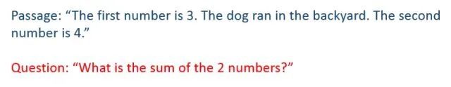
We can see that the middle sentence does not affect the posed question. However, there is a strong connection between the first and third sentences. Using a classic RNN, the hidden state vector at the end of the network may store more information about the sentence concerning the dog rather than the first sentence about the number. Fundamentally, the additional LSTM units increase the likelihood of identifying the correct useful information that should be imported into the hidden state vector.
From a more technical perspective on LSTM units, the unit imports the current word vector xt and outputs the hidden state vector ht. In these units, the construction of ht will be a bit more complex than a typical RNN. The calculations are divided into four components: an input gate, a forget gate, an output gate, and a new storage container.
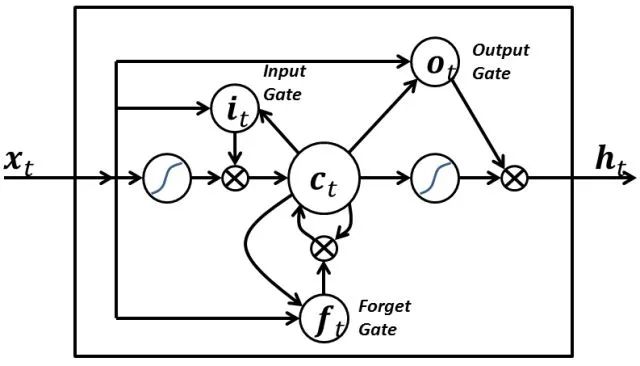
Each gate will use xt and ht (not shown in the figure) as inputs and perform some calculations to obtain intermediate states. Each intermediate state is fed back into different pipelines and ultimately aggregates the information into the form of ht. For simplicity, we will not describe the specific constructions of each gate, but it is worth noting that each gate can be considered a different module within the LSTM, each with different functions. The input gate determines the weights of each input, the forget gate decides what information we will discard, and the output gate determines ht based on the final intermediate state. For more detailed information on the functions of different gates and the complete equations, please refer to Christopher Olah’s blog post (translator’s note: or the Chinese translation).
Referring back to the first example, the question is “What is the sum of the two numbers?” The model must be trained on similar question-answering pairs, and then the LSTM unit will recognize that any sentence without numbers may not affect the answer to the question, thus allowing the unit to use its forget gate to discard unnecessary information about the dog while retaining information about the numbers.
Framing Sentiment Analysis as a Deep Learning Problem
As previously mentioned, the task of sentiment analysis is primarily to input a sequence of sentences and determine whether the sentiment is positive, negative, or neutral. We can break down this particular task (and most other NLP tasks) into five different steps.
-
1. Train a word vector generation model (like Word2Vec) or load pre-trained word vectors
-
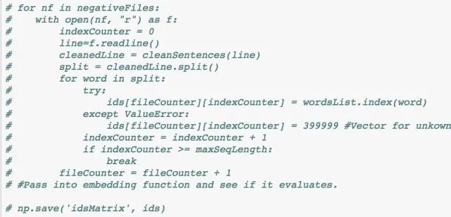
2. Create an ID matrix for our training set (to be discussed later)
-
3. Create the RNN (using LSTM units)
-
4. Train
-
5. Test
Loading Data
First, we need to create word vectors. For simplicity, we will use a pre-trained model.
As the biggest player in the game of machine learning, Google was able to train the Word2Vec model on a massive Google news training set containing over 100 billion different words! From that model, Google was able to create 3 million word vectors, each with a dimension of 300.
Ideally, we would use these vectors, but since the word vector matrix is quite large (3.6GB!), we will use a more manageable matrix trained by a similar word vector generation model called Glove. The matrix will contain 400,000 word vectors, each with a dimension of 50.
We will import two different data structures: one is a Python list of 400,000 words, and the other is a 400,000 x 50 dimensional embedding matrix containing all the word vector values.

To ensure everything has loaded correctly, we can check the dimensions of the vocabulary list and the embedding matrix.

We can also search for a word in the word list, such as “baseball”, and then access its corresponding vector through the embedding matrix.

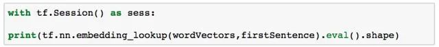
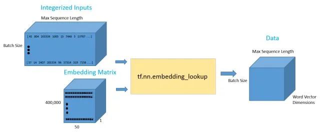
Now that we have our vectors, we will first input a sentence and then construct its vector representation. Suppose we have the input sentence “I thought the movie was incredible and inspiring.” To obtain the word vectors, we can use TensorFlow’s built-in lookup function. This function requires two parameters: one is the embedding matrix (in our case, the word vector matrix), and the other is the ID for each word. The ID vector can be thought of as the integer representation of the training set. This is essentially just the row index for each word. Let’s look at a specific example to clarify.

The data pipeline is illustrated in the following figure.
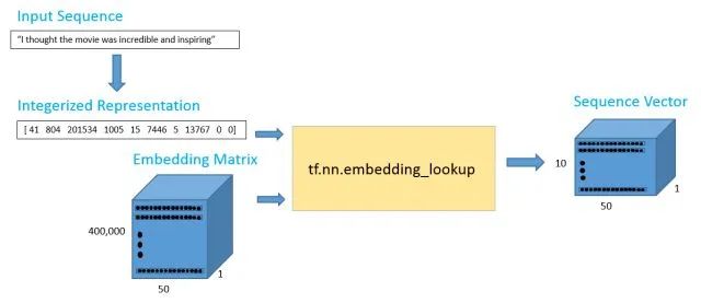
The output of 10 x 50 should contain the 50-dimensional word vector for each of the 10 words in the sequence.
Before creating the ID matrix for the entire training set, let’s take some time to visualize the types of data we have. This will help us determine the best value for setting the maximum sequence length. In the earlier example, we used a maximum length of 10, but this value largely depends on your input.
The training set we will use is the IMDB movie review dataset. This collection contains 25,000 movie reviews, with 12,500 positive reviews and 12,500 negative reviews. Each review is stored in a txt file that we need to parse. The following code will determine the average word count and total for each review.
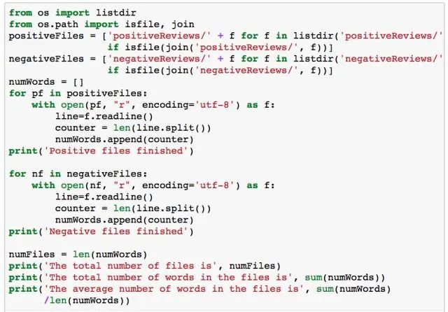
We can also visualize the data using the Matplotlib library in the form of a histogram.
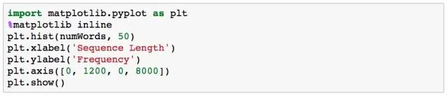
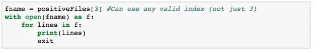
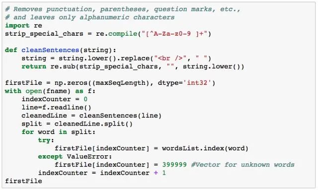
From the histogram and the average word count per file, we can determine that most reviews are under 250 words, at which point we set the maximum sequence length value. maxSeqLength = 250 The following will show how to convert a single file into an ID matrix. Below is a review that looks like a text file format.
Now, convert it into an ID matrix.
Now, do the same for our 25,000 reviews. Load the movie training set and organize it into a 25,000 x 250 matrix. This is a computationally expensive process, so you do not need to run the entire program again; we will load the precomputed ID matrix.


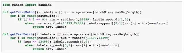
Utility Functions
Below you will find some utility functions that will be useful during the subsequent training process of the neural network.
RNN Model
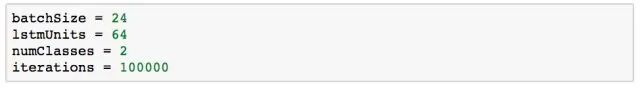
Now we are ready to start creating our TensorFlow graph. First, we need to define some hyperparameters, such as batch size, number of LSTM units, number of output classes, and number of training iterations.
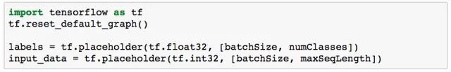
As with most TensorFlow graphs, we now need to specify two placeholders, one for input into the network and one for labels. The most important part of defining these placeholders is understanding the dimensions of each.
The label placeholder is a set of values, each being [1, 0] or [0, 1], depending on whether each training example is positive or negative. Each row in the input placeholder represents the integer representation of each training example included in our batch.
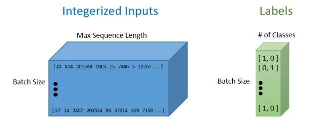
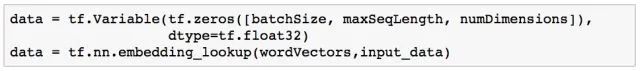
Once we have the input data placeholder, we will call the tf.nn.lookup() function to get the word vectors. Calling this function will return a 3-D tensor of batch size (the number of examples in our batch) up to the maximum sequence length based on the dimensions of the word vectors. To visualize this 3-D tensor, you can simply think of each data point in the integerized input tensor as corresponding to its relevant D-dimensional vector.
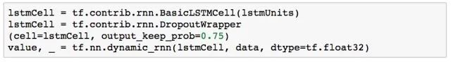
Now that we have the data in the desired form, let’s see how to feed this input into the LSTM network. We will call the tf.nn.rnn_cell.BasicLSTMCell function. This function takes an integer representing the number of LSTM units we want to use. This is one of the hyperparameters adjusted to find the optimal values. Then we will wrap the LSTM units in a dropout layer to prevent the network from overfitting.
Finally, we will feed the LSTM units filled with input data and the 3-D tensor into a function called tf.nn.dynamic_rnn. This function is responsible for unfolding the entire network and creating paths for data to flow through the RNN graph.
As a note, another more advanced network architecture option is to stack multiple LSTM neurons on top of each other. This means that the last hidden state vector of the first LSTM neuron feeds into the second LSTM neuron. Stacking these neurons is a great way to help the model retain more long-term information, but it also introduces more parameters into the model, which may increase training time, require more training samples, and increase the probability of overfitting. For more information on how to stack LSTMs into your model, please refer to the TensorFlow documentation.
The first output of the dynamic RNN function can be thought of as the last hidden state vector. This vector will be reshaped and then multiplied by the final weight matrix and bias term to obtain the final output value.
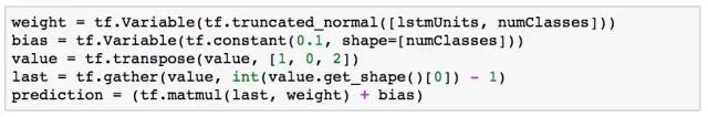
Next, we will define the correct predictions and accuracy metrics to track the performance of the network. The correct prediction formula works by looking at the index of the maximum value of the two output values and then checking if it matches the training labels.

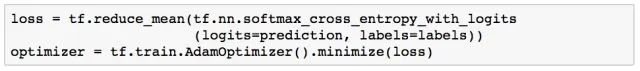
We will define the standard cross-entropy based on the final predicted values, using the Adam optimizer with a default learning rate of 0.01.
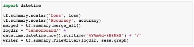
If you want to use TensorBoard to display the values of loss and accuracy, you can also run and modify the following code.
Hyperparameter Tuning
Selecting the correct values for your hyperparameters is a key part of effectively training deep neural networks. You will find that your training loss curve may vary based on the optimizer you choose (Adam, Adadelta, SGD, etc.), learning rate, and network architecture. Especially when using RNNs and LSTMs, there are some other important factors to consider, including the number of LSTM units and the size of the word vectors.
-
Due to the large number of time steps, RNNs are notoriously difficult to train. The learning rate becomes very important as we do not want the weight values to fluctuate due to a high learning rate, nor do we want to train slowly due to a low learning rate. A default value of 0.001 is a good starting point; if the training loss changes very slowly, you should increase this value, and if the loss is unstable, you should decrease it.
-
Optimizer: There is no consensus among researchers on a preferred choice, but Adam is popular due to its adaptive learning rate property (remember, tuning the learning rate may differ depending on the optimizer chosen).
-
Number of LSTM units: This value largely depends on the average length of the input text. While more units allow the model to express more effectively and store more information for longer texts, the network will take longer to train and incur higher computational costs.
-
Word vector size: The dimensions of word vectors typically range from 50 to 300. Larger sizes mean that word vectors can encapsulate more information about the word, but the model will also require more computational resources.
Training
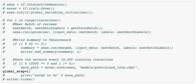
The basic idea of the training loop is to first define a TensorFlow session, then load a batch of reviews along with their associated labels. Next, we call the session’s run function, which has two parameters: the first is called the “fetches” parameter, which defines the expected values we want to compute, and we want the optimizer to calculate since this is the component that minimizes the loss function. The second parameter requires us to input our feed_dict, which is where we provide input for all placeholders. We need to provide batches of reviews and labels, and this loop will repeat over a set of training iterators.
We will load a pre-trained model instead of training the network on this notebook (which would take hours).
If you decide to train this model on your machine, you can use TensorBoard to track the training process. When the following code is running, use your terminal to navigate to the execution directory of this code, enter tensorboard –logdir=tensorboard, and access http://localhost:6006/ in your browser to keep an eye on the training process.
Loading Pre-trained Models
Our pre-trained model’s accuracy and loss curves during the training process are shown below.
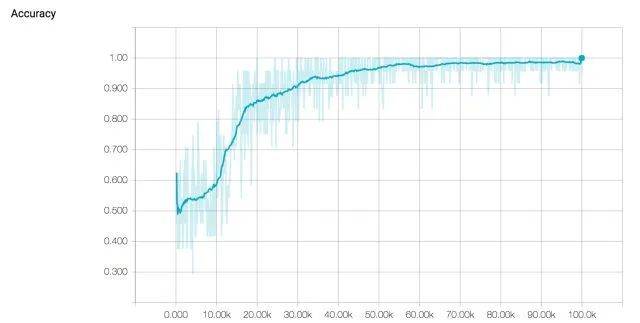
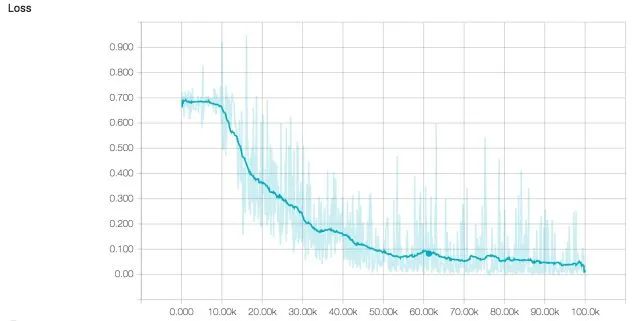
Looking at the training curves above, it seems that the model is progressing well. The loss steadily decreases, and the accuracy approaches 100%. However, when analyzing the training curves, we should also pay special attention to the possibility of the model overfitting the training dataset. Overfitting is a common phenomenon in machine learning where the model becomes too tailored to the training data and loses the ability to generalize to the test set. This means that training a network to reach a 0 training loss may not be the best way to obtain a model that performs well on an unseen dataset. Early stopping is an intuitive technique commonly applied to LSTM networks to address overfitting. The basic idea is to train the model on the training set while also measuring its performance on the test set repeatedly. Once the test error stops steadily decreasing and starts to increase, we know to stop training as this is a signal that the neural network is beginning to overfit.
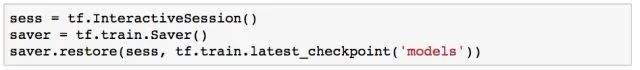
Loading a pre-trained model involves defining another TensorFlow session, creating a Saver object, and then calling the restore function with that object. This function takes two parameters, one for the current session and the other for the name of the saved model.
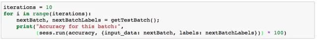
Then we will load some movie reviews from the test set, noting that these reviews have never been seen by the model during training. Running the following code will allow you to see the precision of each batch of tests.
Conclusion
In this note, we conducted an in-depth study of sentiment analysis. We explored the different components involved in the entire process, and then studied the process of writing TensorFlow code to implement the model in practice. Finally, we trained and tested the model to be able to classify movie reviews.
With the help of TensorFlow, you can create your own sentiment classifier to understand a vast amount of natural language and use the results to form compelling arguments. Thank you for reading.
Exciting! The Yi Zhen Natural Language Processing – Academic WeChat Group has been established
You can scan the QR code below, and the assistant will invite you to join the group for communication.
Note: Please modify the remarks to [School/Company + Name + Direction] when adding.
For example – Harbin Institute of Technology + Zhang San + Dialogue System.
Account owner, please avoid adding if you are a micro-business. Thank you!

Recommended Reading:
PyTorch Cookbook (Common Code Snippet Collection)

Easy to Understand! Implementing Transformer with Excel and TF!

Multi-task Learning in Deep Learning - Keras Implementation