This article is a work by Professor Rufin VanRullen from the Université de Toulouse, published in Communications Biology in 2019, titled “Reconstructing faces from fMRI patterns using deep generative neural networks“. DOI: 10.1038/s42003-019-0438-y.
Abstract
Despite reliably decoding different categories from fMRI brain responses, distinguishing visually similar inputs, such as different faces, has proven more challenging. Here, we apply a recently developed deep learning system to reconstruct facial images from human fMRI data. We trained a Variational Autoencoder (VAE) neural network using an unsupervised Generative Adversarial Network (GAN) program on a large dataset of celebrity faces. The latent space of the autoencoder provides a meaningful, topologically organized 1024-dimensional description for each image. We then presented thousands of faces to human subjects and learned a simple linear mapping between multivoxel fMRI activation patterns and the 1024 latent dimensions. Finally, we applied this mapping to new test images, converting fMRI patterns into VAE latent encodings, which were then encoded into facial reconstructions. The system not only performed robust paired decoding (>95% accuracy) but also accurately classified gender and even decoded which face was imagined, rather than seen.
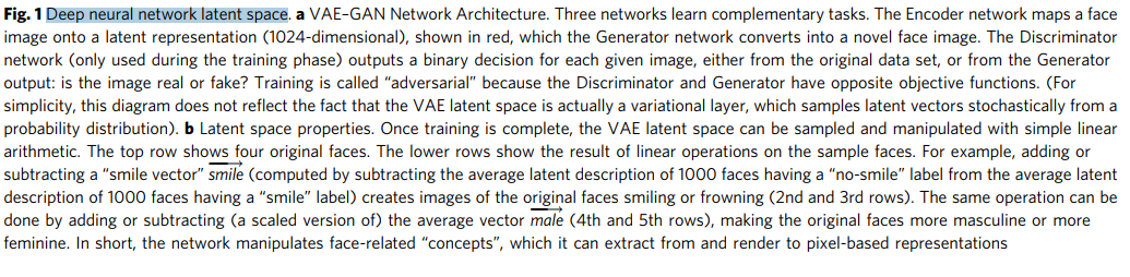
Decoding sensory inputs from brain activity is both a modern technical challenge and a fundamental neuroscience endeavor. Multivoxel pattern analysis of functional magnetic resonance imaging (fMRI), inspired by machine learning methods, has yielded impressive “mind-reading” feats over the past 15 years. However, a well-known challenge is distinguishing brain activity patterns caused by visually similar inputs, such as objects from the same category or different faces. Here, we propose to leverage the latest developments in deep learning. Specifically, we employ a Variational Autoencoder (VAE) trained via a Generative Adversarial Network (GAN) program, as shown in Fig. 1a. The resulting VAE-GAN model is a state-of-the-art deep generative neural network for face representation, processing, and reconstruction. The network’s “face latent space” provides descriptions of many facial features that can be approximated to facial representations in the human brain. In this latent space, faces and facial features (e.g., male) can be characterized as linear combinations of one another and can be manipulated to process different concepts (e.g., male, smiling) using simple linear operations (Fig. 1b). The versatility of this deep generative neural network’s latent space suggests a possible homology with facial representations in the human brain, making it an ideal candidate for fMRI-based face decoding. Therefore, we have ample reason to believe that learning the mapping between the fMRI pattern space and this latent space, rather than the image pixel space (or linear combinations of those pixels, as in recent state-of-the-art methods involving PCA), will yield better results when decoding brain activity. Specifically, we hypothesize that the VAE-GAN model captures and unravels much of the complexity of facial representations, flattening and regularizing the “face manifold,” as the human brain might do, such that simple linear brain decoding methods suffice. Under this hypothesis, we find that this technique outperforms current (non-deep learning) state-of-the-art methods, allowing us to not only reconstruct reliable estimates of seen faces but also decode facial gender or mental imagery. In summary, our contributions are at least threefold. First, we introduce a novel, state-of-the-art brain decoding method based on recent developments in deep learning and generative models. Second, we suggest that this method, along with our large (publicly available) fMRI dataset, can address many prominent questions regarding facial processing in the human brain. We illustrate this proposal with two examples: gender processing and mental imagery, in both cases exceeding previous state-of-the-art results. Third, we speculate that the latent space of deep generative models may be homologous to human brain representations.

VAE architecture and GAN training
We trained a 15-epoch VAE deep network (13 layers) on a labeled database of 202,599 celebrity faces (CelebA dataset) using an unsupervised GAN program. Details of the network architecture are provided in Supplementary Table 1, and training process details can be found in previous studies. During GAN training, three sub-networks learn complementary tasks (Fig. 1a). The encoding network learns to map facial images to a 1024-dimensional latent representation (Fig.1 in red), while the generating network is used to produce new facial images; the encoder’s learning objective is to make the output facial image as close to the original image as possible (this reconstruction objective is measured as the L2 loss in the feature space of the discriminator network, as described in the references). The generating network learns to convert latent 1024-dimensional vectors in the latent space into plausible facial images. The discriminator network (six layers, used only during training) learns to generate a binary decision for each given image (from the original dataset or from the generator’s output): Is the image real or fake? The discriminator and generator have opposing objective functions and update in alternating steps: if the discriminator can reliably determine which images come from the generator (fake) and which come from the dataset (real), the discriminator is rewarded; if the generator can produce images that the discriminator network cannot classify correctly, the generator is rewarded. At the end of training, the discriminator network is discarded, and the encoding/generating network is used as a standard (variational) autoencoder. Specifically, we use the encoder to generate 1024-D latent encodings for each input facial image shown to human subjects, which serve as design matrices for fMRI GLM (General Linear Model) analysis (see below in the “Brain Decoding” section). We use the generator to reconstruct facial images based on the output (1024-dimensional latent vector estimates) of the “Brain Decoding” system.
As Cowen et al. described, Principal Component Analysis (PCA) was used as a baseline (linear) model for face decomposition and reconstruction. By retaining only the first 1024 principal components (PCs), each image can be converted into a 1024-dimensional encoding to train our brain decoding system (as described below), and the output encoding can be transformed back into facial images for visualization using inverse PCA transformation. The baseline model and some of its properties are illustrated in Supplementary Fig. 1.
The study included four subjects (males, ages 24-44), conducted according to national ethical regulations. Subjects provided informed consent. Functional MRI data were collected on a 3T Philips ACHIEVA scanner (gradient echo pulse sequence, TR = 2 s, TE = 10 ms, 41 slices with a 32-channel head coil, slice thickness = 3 mm with a 0.2 mm gap, in-plane voxel dimensions 3 × 3 mm). The slices were positioned to cover the entire temporal and occipital lobes. High-resolution anatomical images were also acquired per subject (1 × 1 × 1 mm voxels, TR = 8.13 ms, TE = 3.74 ms, 170 sagittal slices).
Each subject was tested in eight scanning sessions. In each scanning session, subjects underwent 10 to 14 facial runs. Each facial run began and ended with a 6-second blank interval. Subjects were presented with 88 facial stimuli. Each face was presented for 1 second, followed by a 2-second stimulus interval (i.e., trial interval of 3 seconds). These faces were presented from an eight-degree angle and shown in the center of the screen. Among the 88 facial stimuli for each run, 10 test faces (5 male and 5 female) were randomly interspersed. In alternating runs, a different set of 10 test faces was presented (i.e., 20 test faces for each subject). Each run also included 30 invalid “fixation” trials, during which a fixation cross was displayed instead of facial stimuli. The facial images presented to subjects in the scanner were encoded once through the VAE-GAN autoencoder—this was done to ensure that the recorded brain responses focused on the facial or background image properties that could be reliably extracted and reconstructed by the deep generative network. The training image set for each subject was randomly drawn from the CelebA dataset, with an equal number of male and female faces for each run, and the training sets for different subjects did not overlap. Initially, a different pool of 1000 potential test faces was randomly drawn for each subject; then, we manually selected 10 male and 10 female faces from this pool, with varying ages, skin tones, poses, and emotions. Similarly, these 20 test faces were different across subjects. To keep subjects alert and encourage them to pay attention to facial stimuli, they were asked to perform a “1-back” comparison task: pressing a button as quickly as possible whenever the facial image matched the previous face. In addition to the 88 facial trials, each run included 8 one-back trials, where repeated images were discarded from the brain decoder training process (as described below). Furthermore, whenever the sequence of facial images was replaced by a large static gray square in the center of the screen (lasting 12 seconds), subjects were instructed to imagine a specific face they had previously chosen from a set of 20 possible faces. For each subject, only one face was chosen and studied in detail (outside the scanner, between scanning sessions 4 and 5) and was then repeatedly imagined throughout scanning sessions 5-8. In odd (versus even) scanning runs, unique 12-second image trials were introduced at the start (versus end) of the run. Among the four experimental subjects, the number of recorded image trials varied from 51 to 55 (mean 52). Each image trial was followed by a 6-second blank period.
fMRI data were processed using SPM 12. For the data from each participant in each scanning session, temporal slice timing correction and registration were performed. Each session was then co-registered to the T1 scan of the second MRI session. Data were not normalized or smoothed. The onset and duration of each trial (fixation, training face, test face, one-back or imagery) were input as regressors into the General Linear Model (GLM). Alternatively, the 1024-dimensional latent vectors of the training facial images (from VAE-GAN or PCA models) could be modeled as parametric regressors. Motion parameters were input as nuisance regressors. Before estimating GLM parameters, the entire design matrix was convolved with SPM’s canonical hemodynamic response function (HRF).
We trained a simple brain decoder (linear regression) to associate the 1024-dimensional latent representations of facial images (obtained by running images through the “Encoder” as shown in Fig.1 or using PCA decomposition, as described above and in Supplementary Fig. 1) with the corresponding brain response patterns recorded when human subjects viewed the same faces in the scanner. The process is illustrated in Fig.2a. In a rapid event-related design, each subject saw over 8000 faces on average, and we used the VAE-GAN latent dimensions (or image projections on the first 1024 PCs) as 1024 parametric regressors for the BOLD signal (see the fMRI analysis section above). These parametric regressors can be positive or negative (since the VAE training objective tends to yield VAE-GAN latent variables that are approximately normally distributed). An additional classification regressor (“face versus fixation” contrast) was added to the model as a constant “bias” term. We verified that the design matrix was “full rank”, meaning all regressors were linearly independent. This property is expected, as VAE-GAN (and PCA) latent variables tend to be uncorrelated. The linear regression performed by the SPM GLM analysis thus yields a weight matrix W (1025 x nvoxels dimensions, where nvoxels is the number of voxels in the brain ROI) optimized to predict brain patterns in response to training face stimuli.
In mathematical terms, we assume a linear mapping W exists between the 1025-dimensional latent vector X (including the bias term) and the corresponding brain activation vector Y (length nvoxels) such that:

Training the brain decoder involves finding the optimal mapping W by solving for W:

where X T X is the covariance matrix of the latent vectors used for training (1025 x 1025 dimensions).
To use this brain decoder during the “testing phase”, we simply reverse the linear system, as shown in Fig.2b. We presented 20 new test faces (not seen during the training phase) to the same subjects. Each test face was presented on average 52.8 times (subject range: 45.4-55.8, interleaved randomly with training facial images) to enhance the signal-to-noise ratio. The resulting brain activity patterns were simply multiplied by the transposed weight matrix W T (nvoxels by 1025 dimensions) and its inverse covariance matrix to produce estimates of the 1024 latent face dimensions (in addition to an estimate of the bias term, which is no longer used). We then used the generator network (as shown in Fig.1) to convert the predicted latent vectors into reconstructed facial images. For the baseline PCA model, the same logic was applied, but facial reconstruction was obtained through the inverse PCA of the decoded 1024-dimensional vector.
In mathematical terms, testing the brain decoder involves retrieving the latent vector X for each new brain activation pattern Y using the learned weights W. Starting from Eq.1, we now solve for X:

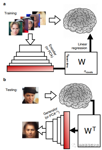
Fig.2 Brain decoding of face images based on VAE–GAN latent representations. a Training phase. Each subject saw ~ 8000 faces (one presentation each) in a rapid event-related design. The same face images were also run through the “Encoder” network (as described in Fig. 1) or a PCA decomposition, to obtain a 1024-dimensional latent face description. The “brain decoder” was a simple linear regression, trained to associate the 1024-dimensional latent vector with the corresponding brain response pattern. This linear regression, with 1024 parametric regressors for the BOLD signal (and an additional constant “bias” term), produced a weight matrix W (1025 by nvoxels dimensions) optimized to predict brain patterns in response to face stimuli. b Testing phase. We also presented 20 distinct “test” faces (not part of the training set; at least 45 randomly interleaved presentations each) to the subjects. The resulting brain activity patterns were simply multiplied by the transposed weight matrix WT (nvoxels by 1025 dimensions) and its inverse covariance matrix to produce a linear estimate of the latent face dimensions. The Generator network (Fig. 1a) or an inverse PCA transform was then applied to translate the predicted latent vector into a reconstructed face image
The image quality comparisons between VAE-GAN and PCA face reconstructions were obtained through human judgments acquired via Amazon Mechanical Turk (AMT) against financial compensation. Each of the 20 test images from four subjects was displayed under the label “original”, followed by the VAE-GAN and PCA-based reconstructions, respectively displayed under “Option A” and “Option B” (with inter-observer balanced A/B distribution). The instructions read: “Which of the two modified faces looks most like the original? Choose A or B.” Each pair of images was compared a total of 15 times, with at least 10 different AMT “workers” viewing each response assignment (the VAE-GAN/PCA of Option A/B) with at least five workers per response. Thus, the experiment led to a total of 1200 comparisons (= 4 × 20 × 15) between the two facial reconstruction models.
Statistics and reproducibility
The accuracy of brain decoding was compared to chance probabilities in two ways. A “full identification” test was successful only when the brain-estimated latent vector was closer to the target image’s latent vector than all 19 distractor image latent vectors (measured by Pearson correlation). Each subject’s p value was derived from a binomial test with parameters: probability = 1/20, draws = 20. The “paired identification” test involved comparing the brain-estimated latent vector with its target image latent vector and those of randomly selected distractor image latent vectors; identification was successful whenever the brain-estimated latent vector was closer to the target (Pearson correlation) than to the distractor. Since the continuous testing of a given target is not independent, the binomial test is not appropriate here (and often overestimates significance). Instead, we employed a non-parametric Monte Carlo test: based on the null hypothesis, the ranks of the brain-estimated latent vector among the 20 (Pearson) correlations with the test image latent vectors could take any value between 1 and 20 (the binomial test would assume that intermediate ranks are more likely). We performed 106 random uniform draws of the ranks among the 20, and used these draws to compute an alternative distribution of decoding performance values under the null hypothesis. For each subject, the p value was the (upper) percentile of decoding performance within that distribution. (We verified, as expected, that this produced more conservative significance values than the parameter-based binomial test: probability = 1/2, draws = 20 × 19).
For both “full” and “paired” recognition measurements, we compared group-level performance of the VAE-GAN and PCA models using the Friedman nonparametric test. The Friedman test, used for subsequent post hoc comparisons, was also applied to compare the gender decoding performance of three anatomical voxel selections for each decoding model (VAE-GAN or PCA).
Perceptual comparison measurements (the proportion of VAE-GAN selections) were compared to the null hypothesis (equal likelihood of selecting VAE-GAN and PCA reconstructions) using a binomial test with parameters: probability = 1/2, draws = 4 × 20 × 15 (four fMRI subjects, each with 20 test images, each with 15 comparisons). A binomial test with parameters was also used to compare the individual and group-level gender decoding performance against the probability of chance occurrence (50%): probability = 1/2, draws for individual tests = 20, group-level tests = 4 × 20 (four subjects, each with 20 test images). The Friedman test, used for subsequent post hoc comparisons, was used to compare the gender decoding performance of three anatomical voxel selections.
As described above, image decoding performance was measured in a paired fashion (“paired recognition”): the brain-estimated latent vector was correlated with the true (ground-truth) latent vector and 19 distractor latent vectors using Pearson correlation; decoding accuracy is the proportion of distractor correlations that fall below the true correlation. This performance was averaged across subjects and compared to chance probability (50%) using the same Monte Carlo nonparametric test as above: this time, all 204 = 160,000 possible draws could be explicitly considered (four subjects, each with ranks from 1 to 20) to create an alternative distribution to compare against group-level performance values. The Friedman test, used for subsequent post hoc comparisons, was applied to compare the image decoding performance of three anatomical voxel selections.
The source data used to generate Figs. 4 b,c,5,6 and 7 are available in Supplementary Data 1.
Results
Face decoding and reconstruction
We used the pre-trained VAE-GAN model described in Fig.1 (using “frozen” parameters) to train the brain decoding system. During training (Fig.2a), the system learned the correspondence between brain activity patterns in response to a large number of facial images and the corresponding 1024-dimensional latent representations of the same faces in the VAE network. An average of over 8000 different examples (across subjects: 7664-8626) were involved, with each subject undergoing 12 hours of scanning across eight separate sessions. The learning process assumed that the activation of each brain voxel could be described as a weighted sum of the 1024 latent parameters, and we simply estimated the corresponding weights through linear regression (using the GLM function in SPM; see Methods). After training (Fig. 2b), we reversed the linear system so that the decoder could receive specific new facial images (not included in the training set) as input, yielding output as a 1024-dimensional latent feature vector for that face. This was then generated (or “reconstructed”) into facial images via the (VAE-GAN) neural network.
We compared the results obtained from this deep neural network model with those produced by another simpler facial image decomposition model: Principal Component Analysis (PCA, retaining only the first 1024 principal components from the training dataset; see Supplementary Fig. 1). The PCA model also describes each face with a 1024-dimensional vector in the latent space and can also be used to reconstruct faces based on estimates of this 1024-dimensional feature vector, as shown in recent studies.
For both the deep neural network and PCA-based models, we defined a subset of gray matter voxels as our “regions of interest” (ROIs). In fact, many parts of the brain perform computations unrelated to facial processing or recognition; entering these regions in our analysis would adversely affect the signal-to-noise ratio. Our selection criteria combined two factors: (i) voxels that were expected to respond to facial stimuli (as determined by t-tests between facial and baseline conditions, i.e., fixation on a blank screen), and (ii) voxels whose BOLD response variance was expected to improve when the 1024 latent facial features were entered as regressors into the linear model (compared to a baseline model with only one binary face regressor: presence/absence of a face). Supplementary Fig. 2 illustrates the distribution of voxels along these two dimensions and the corresponding selection criteria for a representative subject. Among the four subjects, the number of voxels produced by the selection was approximately 100,000 (mean: 106,612; range: 74,388-162,388). The selected voxels are shown in Fig.3; they include occipital, temporal, parietal, and frontal regions. Separate selections were made based on the PCA facial parameters and used for the PCA-based “brain decoder” (mean of selected voxels: 106,685; range: 74,073–164,524); the selected regions for both models were nearly identical. It is important to emphasize that the voxel selection criteria described above were based solely on the BOLD responses to the training facial images, not to the 20 test images; thus, the decoding analysis does not suffer from circular reasoning issues caused by this voxel selection.
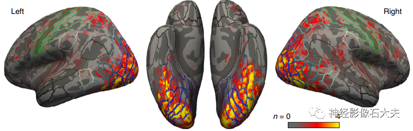
Fig. 3 Voxels selected for brain decoding. Voxels were selected based on a combination of their visual responsiveness and their GLM goodness-of-fit during the brain decoder training stage (Fig. 2a). The color code (red to yellow) indicates the number of subjects (1–4) for whom each particular voxel was selected. The colored lines indicate the boundaries of standard cortical regions.
Each subject’s test image set reconstructed facial images is illustrated in Fig.4a. Although both the VAE-GAN and PCA models can reconstruct faces with acceptable similarity to the original, the images reconstructed from the deep generative neural network (VAE-GAN) appear more realistic and closer to the original images. We quantified the performance of our brain decoding system by correlating the latent vectors of the 20 test faces estimated by the brain with the true vectors from the actual test images and another test image (distractor): if the correlation with the true target vector was higher than with the distractor vector, the brain decoding was considered “correct.” This was repeated for all (20 × 19) pairs of test images, and non-parametric Monte Carlo tests were applied to compare the average performance against chance probability (50%) (see Methods: Statistics). The GAN model achieved 95.5% classification accuracy (range: 91.3–98.7%, all p <10e-6), while the PCA model reached only 87.5% (range 76.6-92.4%, still significantly above chance, all p <10e-4, but far below the GAN model; Friedman nonparametric test, χ²(1) = 4, p < 0.05). We also tested the brain decoder’s ability to pick the correct face from the 20 test faces: this “full identification” task was successful only when the reconstructed latent vector correlated with the true target vector higher than all 19 distractor vectors. This was a stricter face recognition test, with a probability of 5%: the VAE-GAN model achieved a correct rate of 65% (range: 40-75%, binomial test, all p < 10e-6), while the PCA model only had a correct identification rate of 41.25% (range 25–50%, all p < 10e-3); similarly, the VAE-GAN model’s performance was significantly better than that of PCA (χ²(1) = 4, p < 0.05).
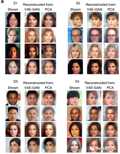
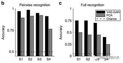
Fig.4 Face reconstruction. a Examples of reconstructed face images. For each of our four subjects (S1–4), the first column displays four example faces (two male+two female, chosen among the 20 test faces) actually shown to the subject during the scanning sessions. The next two columns are the face reconstructions based on the corresponding fMRI activation patterns for the brain-decoding system trained using the VAE–GAN latent space (middle column) or PCA decomposition (right column). b Pairwise recognition. The quality of brain decoding was quantified with a pairwise pattern classification (operating on the latent vector estimates), and the average performance compared with chance (50%). Brain decoding from the VAE–GAN model achieved 95.5% correct performance on average (p < 10e-6), the PCA model only 87.5% (p < 10e−4); the difference between the two models was significant (χ2(1) = 4, p < 0.05). c Full recognition. A more-stringent performance criterion was also applied, whereby decoding was considered correct if and only if the procedure identified the exact target face among all 20 test faces (chance = 5%). Here again, performance of the VAE–GAN model (65%) was far above chance (p < 10e−6), and outperformed (χ2(1) = 4, p < 0.05) the PCA model (41.25%; p < 10e−3)
Since linear regression models typically require more data samples than their input dimensions, we initially decided to train the brain decoding system with approximately 8000 faces per subject (compared to 1024 latent dimensions). To determine whether a smaller training set would suffice, we repeated the linear regression steps (calculating the W matrix in Fig. 2) using only half, a quarter, or an eighth of the training dataset (see Supplementary Fig. 3). For both paired and full recognition measurements, using approximately 1000 training faces already yielded performance above chance probability; however, decoding performance continued to grow with increasing training set size, peaking at around 8000 training faces. Importantly, for all training set sizes, the PCA model consistently performed below the VAE-GAN model.
These comparisons suggest that creating a linear mapping from brain activation to VAE-GAN latent space is easier and more effective than to PCA space. This aligns with our hypothesis that deep generative neural networks are more similar to the spatial representation of faces. Moreover, this classification accuracy is measured based on the distances (or vector correlations) in the latent space of each model; if their accuracy is assessed using common metrics (e.g., perceptual quality of reconstructed images), it may even exacerbate the differences between the two models. To support this idea, we asked human observers participating in the experiment for the first time to compare the quality of faces reconstructed from the two models: each original test image from four subjects was displayed alongside its corresponding VAE-GAN and PCA reconstructions; observers decided which reconstruction appeared more similar to the original. At least 10 different participants scored each pair 15 times, with at least 5 participants viewing the two response options in arbitrary order, first VAE-GAN or PCA. 76.1% of trials selected the VAE-GAN reconstruction, while only 23.9% selected the PCA reconstruction. In other words, observers were three times more likely to prefer the quality of VAE-GAN reconstructions than PCA reconstructions, and this difference is highly unlikely to have occurred by chance (binomial test, 1200 observations, observers decided which reconstruction perceptually resembled the original more closely. At least 10 different participants scored each pair 15 times, with at least 5 participants viewing the two response options in arbitrary order, first VAE-GAN or PCA. 76.1% of trials selected the VAE-GAN reconstruction, while only 23.9% selected the PCA reconstruction. In other words, observers were three times more likely to prefer the quality of VAE-GAN reconstructions than PCA reconstructions, and this difference is highly unlikely to have occurred by chance (binomial test, 1200 observations, p < 10e-10).
Contributions from distinct brain regions
To determine which brain regions contributed most to the facial reconstruction capabilities of the two brain decoding models, for each subject, we divided our voxel selection into three equally sized subsets, as shown in Fig.5a. We then applied the brain decoding and facial reconstruction procedures to each of these three subsets separately. The paired recognition results showed that occipital voxels, and to a lesser extent temporal voxels, provided most of the information needed for brain decoding (Fig. 5b). Both models (VAE-GAN: 91.8%, all individual p < 10e-6; PCA: 87.2%, all p < 10e-4) demonstrated decoding performance far exceeding chance probability (50%), and so did the temporal voxels (VAE-GAN: 78.8%, all p < 10e-3; PCA: 73.6%, all p < 0.01). On the other hand, while frontoparietal voxels met our selection criteria (see Fig. 3), they did not carry enough reliable information for accurate classification (VAE-GAN: 60.1%, one subject p < 10e-6, all others p > 0.2; PCA: 56.4%, one subject p < 10e-6, all others p > 0.05). The result patterns of the VAE-GAN and PCA-based decoding models were the same: non-parametric Friedman tests indicated that performance differed among the three subsets (for VAE-GAN: χ²(2) = 8, p < 0.02; for PCA: χ²(2) = 6.5, p < 0.04), and post hoc tests showed that occipital voxels performed significantly better than frontoparietal voxels, with temporal voxels falling in between (with no significant differences from either of the other two). Across all voxel selections, PCA consistently produced lower accuracy than VAE-GAN—though given our limited number of subjects, this difference did not reach statistical significance (for all three voxel selections, χ²(1) ≥ 3, p > 0.08).
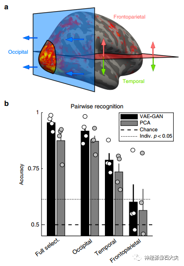
Fig. 5 Contributions from distinct brain regions. a Voxel segmentation procedure. To investigate the brain regions that most strongly supported our brain-decoding performance, while keeping the different subsets comparable, we linearly separated our voxel selection into three equally sized subsets. First, the 1/3 of most posterior voxels for each subject were labeled as “occipital”. Among the remaining voxels, the more rostral half (1/3 of the initial number) was labeled as “temporal”, and the remaining caudal half as “frontoparietal”. This three-way segmentation, different for each subject, was chosen because the performance of our brain-decoding procedure is highly sensitive to the number of included voxels. b Pairwise recognition performance for the different regions of interest. The full selection refers to the set of voxels depicted in Fig. 3; it is the same data as in Fig. 4b, averaged over subjects (error bars reflect standard error of the mean). Circles represent individual subjects’ performance. The dotted line is the p < 0.05 significance threshold for individual subjects’ performance. Among the three subsets, and for both the VAE–GAN and PCA models, performance is maximal in occipital voxels, followed by temporal voxels. Frontoparietal voxels by themselves do not support above-chance performance (except for one of the four subjects). In all cases, the VAE–GAN model performance remains higher than the PCA model.
To further distinguish the relative contributions of the three brain regions to brain decoding performance, we also employed a variance partitioning approach (Supplementary Fig. 4). Consistent with the results already described in Fig.5b, we found that the latent vectors from occipital voxels predicted the largest portion of variance in the corresponding true latent vectors, followed by temporal voxels, and lastly frontoparietal voxels. Each of these three regions also contributed uniquely and independently to the explained variance, which was significantly larger for the VAE-GAN than the PCA model. That is, while occipital voxels provided the most accurate reconstructions, temporal voxels conveyed not just redundant information.
Finally, another way to study the brain representations of specific facial attributes is to create a simple classifier that labels the brain-decoded latent vectors based on that facial attribute. This is illustrated in Fig. 6 , again taking the “gender” facial attribute as an example. Each brain-decoded latent vector was projected onto the “gender” axis in the latent space (Fig.6a), with the sign of the projection determining the classification output (“male” for positive, “female” for negative). This basic classifier provided enough information to classify facial gender with 70% accuracy (binomial test, p = 0.0001; Fig. 6b). Non-parametric Friedman tests indicated differences in gender decoding performance among the three voxel subsets (χ²(2) = 7.6, p < 0.03), with post hoc tests showing that occipital voxels performed significantly better than frontoparietal voxels, with temporal voxels falling in between (with no significant differences from the other two). Previous attempts to classify facial gender using multivoxel pattern analysis achieved limited success, with maximum classification accuracies below 60%. Our simple linear brain decoder (Fig.6a) has improved upon these previous methods while still leaving room for future enhancements, such as employing more powerful classification techniques (e.g., SVM) on the brain-decoded latent vectors.
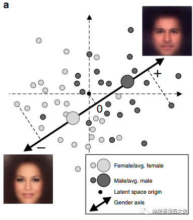
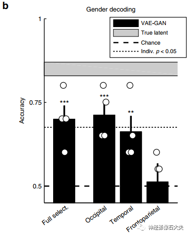
Fig. 6 Gender decoding. a Basic linear classifier. A simple gender classifier was implemented as a proof-of-principle. The “gender” axis was computed by subtracting the average latent description of 10,000 female faces from the average latent description of 10,000 male faces. Each latent vector was simply projected onto this “gender” axis, and positive projections were classified as male, negative projections as female. b Decoding accuracy. When applied to the true latent vectors for each subject’s test faces, this basic classifier performed at 85% correct (range: 80–90%). This is the classifier’s ceiling performance, represented as a horizontal gray region (mean ± sem across subjects). When operating on the latent vectors estimated via our brain-decoding procedure, the same gender classifier performed at 70% correct, well above chance (binomial test, p = 0.0001; bars represent group-average accuracy ± sem across subjects, circles represent individual subjects’ performance). Gender classification was also accurate when restricting the analysis to occipital voxels (71.25%, p = 0.00005) or temporal voxels (66.25%, p < 0.001), but not frontoparietal voxels (51.25%, p = 0.37). The star symbols indicate group-level significance: ***p < 0.001, **p < 0.01. The dotted line is the p < 0.05 significance threshold for individual subjects’ performance.
To further demonstrate the versatility of our brain decoding method, we next applied it to another well-known challenging problem: retrieving information about stimuli that subjects have not directly experienced, but only imagined in their “mind’s eye.” Previous research has shown that this classification problem can be solved when the different categories of stimuli to be imagined are visually distinct, such as images from different categories. However, to our knowledge, the ability to distinguish highly visually similar objects (e.g., different faces) during the imagery process has not been reported before.
Before the experiment, each subject selected one face from a set of 20 possible images (different from their training and testing image sets). During the experiment, they were asked to imagine this specific face whenever a gray square appeared in the center of the screen (displayed for 12 seconds). During fMRI scanning, these imagery trials were averaged 52 times (subject range: 51-55), interleaved with normal stimulus presentations. The average BOLD response during the imagery was then used to estimate the latent face vector (using the brain decoder illustrated in Fig 2b), and this vector was compared in pairs with the 20 possible latent vectors as described for the previous test images (Figs. 4b, 5b). As shown in Fig. 7 (see also Supplementary Fig. 6), in each of our predefined regions of interest (full selection p = 0.53, occipital p = 0.30 or frontoparietal p = 0.43), paired decoding performance did not differ from chance (50%), with the temporal voxel selection being the only exception, yielding 84.2% correct decoding (p = 0.012). Non-parametric Friedman tests indicated differences in imagery decoding performance among the three subsets (χ²(2) = 6.5, p < 0.04), with post hoc tests showing that temporal voxels performed significantly better than frontoparietal voxels, while occipital voxels fell in between (with no significant differences from the other two). Overall, the temporal region, but not occipital or frontoparietal regions, could support mental imagery reconstruction. This performance may reflect the strong involvement of temporal brain regions in high-level face processing, as well as the predominantly top-down nature of mental imagery. Regardless, the ability to classify imagined faces from brain response patterns once again highlights the flexibility and potential of our method.
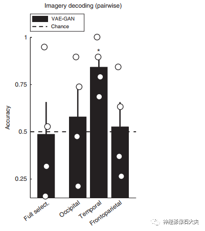
Fig. 7 Imagery decoding. The fMRI BOLD response pattern recorded during mental imagery of a specific face (not visible on the screen) was passed through our brain-decoding system. The resulting estimated latent vector was compared with the true vector and 19 distractor vectors, in a pairwise manner. Only the temporal voxel selection supported above-chance imagery decoding, with 84.2% correct performance (p = 0.012). Neither occipital, nor frontoparietal regions, nor the full voxel selection performed above chance (all p > 0.30). Bars represent group-average accuracy ( ± sem across subjects), circles represent individual subjects’ performance. The star symbols indicate group-level significance: * for p < 0.05.
We found that we can leverage the representational power of deep generative neural networks (especially the VAE combined with GAN) to provide better image spaces for linear brain decoding. Compared to running in pixel space, our approach yielded superior results in both quality and quantity. Specifically, we could reliably distinguish fMRI patterns induced by one face from those induced by another, or determine the gender of each face, a result that has proven elusive thus far. We could even decode faces that were unseen but imagined—this is a true “mind-reading” achievement.
One explanation for the performance of our method may be that the topological structure of the VAE-GAN latent space is very well suited for brain decoding. We know that this space supports linear operations on faces and facial features (Fig. 2). We also know that nearby points in this space can be mapped to visually similar but always plausible faces due to the construction (from the variational training objectives of the VAE and the generative objectives of the GAN). Therefore, this latent space makes brain decoding more robust to small mapping errors, partially explaining the performance of our model. However, beyond these technical considerations, it may simply be that the VAE-GAN latent space is topologically similar to the face representation space in the human brain. The two types of neural networks (artificial neural networks and biological neural networks) may share similar properties, implicit in their objective functions: they have to “unfold” the complexity of face image representation in some way (in other words, flatten the “face manifold”) to facilitate manipulation. While it is unlikely that there is a single solution to this difficult optimization problem (in fact, there may even be an infinite number of solutions), it is conceivable that all effective solutions may share common topological features. This speculation about the homology of human representations and the latent space of deep generative neural networks could be easily tested in the future, for example, using representational similarity analysis. However, it must be clarified that we do not wish to imply that our specific VAE-GAN implementation is unique in its applicability to brain decoding or its similarity to brain representations; rather, we believe that an entire class of deep generative models may share similar properties.
Given the explosive growth of deep generative models in machine learning and computer vision over the past few years, it seems only a matter of time before these methods are successfully applied to brain decoding. In fact, in the past year or so, several methods similar to ours (but with important differences) have been developed and distributed in preprint archives or conference proceedings. Some have used GANs (without associated autoencoders) to generate natural image reconstructions and train brain decoders to associate fMRI response patterns with GAN latent spaces. Others have indeed utilized the latent space of autoencoders (variational or non-variational), but without GAN components. Still, others have attempted to train GANs to directly generate natural image reconstructions from brain responses, rather than using a pretrained latent space on natural images, and only learn the mapping from brain responses to the latent space. All of these pioneering studies have achieved astonishing brain decoding reconstructions of natural scenes or geometric shapes.
Perhaps most comparable to our own method is the one proposed by Güclütürk et al. for reconstructing facial images. They applied GAN training on the outputs of a convolutional encoder trained on the CelebA dataset, a standard ConvNet called VGG-Face, followed by PCA to reduce its dimensionality to 699; then they learned to map brain responses to this PCA “latent space” through Bayesian probability inference (maximum posterior estimation) and used GANs to convert the estimated latent decoding vector into face reconstructions. The test face reconstructions obtained by Güclütürk et al., although using lower image resolution (64 × 64 pixels) compared to our own image reconstructions (128 × 128 pixels), were already remarkable. The authors estimated the reconstruction accuracy using structural similarity measures, yielding a similarity of 46.7% for their model (compared to about 37% for the PCA-based baseline model). In our case, the structural similarity between the original test images and our brain decoding reconstructions reached 50.5% (across subjects: 48.4-52.8%), while our PCA model version still significantly lower, around 45.8% (range: 43.5–47.9%; χ²(1) = 4, p < 0.05). While part of these improvements can be attributed to the higher pixel resolution of our reconstructions, it is clear that the performance of our model is at least as good as that of the model developed concurrently by Güclütürk et al. This is particularly important because our brain decoding method voluntarily remains much simpler: we use a direct linear mapping between brain responses and latent vectors, rather than maximum posterior probability inference. In our view, the burden of absorbing the complexity of facial representations should rest on the generative latent space rather than the brain decoder; an effective space should be topologically similar to human brain representations, thereby providing simple (linear) brain decoding. Thus, the current results reinforce our hypothesis that state-of-the-art generative models, at least in the domain of facial processing, can bring us closer to potential human brain representation models.
The proposed brain decoding model holds great potential for future exploration of facial processing and representation in the human brain. As noted, this model can be used to visualize the facial feature selectivity of any voxel or ROI in the brain—directly displayed as actual facial images. This method can also be used to study the brain representations and perceptions of facial features that are behaviorally and socially important (such as gender, race, emotion, or age); or to investigate the brain’s execution of facial-specific attention, memory, or mental imagery. For example, one important conclusion we explored is that occipital voxels contribute significantly to the decoding of perceived faces (Fig.5), rather than imagined faces (Fig. 7). On the other hand, temporal voxels seem to contribute similarly to both types of trials. This finding may have implications for understanding mental imagery and top-down perceptual mechanisms. To help ensure that these promises are maximally realized, we are making the entire fMRI dataset, the brain decoding models for each of the four subjects, and the deep generative neural networks for facial encoding and reconstruction fully available to the community (see Supplementary Materials for details).
Compiling is not easy, If you find this helpful, please actively share, bookmark, and click “Looking” at the bottom right corner, so more people can see it.
Click “Read the original text” to see more related articles. The original text and supplementary materials can be obtained by contacting the authors.
For those interested in neuroimaging and machine learning, you can scan the code to join the group for communication and learning.:

Welcome to scan the code to follow the neuroimaging Dr. Shi.