Reconstructing Computational System Dynamics Using RNNs

Introduction

Today I would like to share a Perspective paper published in October 2023 in Nature Review Neuroscience by Daniel Durstewitz, Georgia Koppe, and Max Ingo Thurm from Heidelberg University, Germany. The title of the paper is Reconstructing computational system dynamics from neural data with recurrent neural networks.

This article focuses on data-driven reconstruction of neural dynamical systems. It first introduces the basic background of neural dynamical systems and the prerequisites for reconstructing neural dynamical systems using RNNs, describes several different RNN models (Reservoir, Echo State Machines, NeuralODE, SINDy, etc.), and compares the training, evaluation, and performance validation methods of different RNN models, as well as how to explain RNN models as much as possible in the context of neuroscience.

TL;DR:

In the past, computational models in neuroscience were often represented in the form of differential equations, falling under the study of dynamical systems theory (DST), which provides mathematical tools for neural computational models. Recently, machine learning tools such as recurrent neural networks (RNNs) have begun to be used for modeling neural dynamical systems, simulating the nonlinear dynamics of neural and behavioral processes through the underlying systems of differential equations. RNN models can be used to train brain neural activities under recognition tasks in humans and animals, and RNNs can also be used to directly fit neural data, such as physiological and behavioral data, thus directly inheriting the temporal and geometric characteristics within the data. The approach of using RNNs to simulate neural data from animals and humans in experiments is called dynamical system reconstruction. This article will introduce the background, conditions, and methods for using RNNs for dynamical system reconstruction.

Article Background

The realization of cognitive functions is related to neural dynamics:

Theoretical neuroscience suggests that computations in the nervous system can be described based on potential nonlinear system dynamics. On one hand, most physical or biological processes can be represented by differential or difference equations; on the other hand, dynamical systems are computationally universal and can operate on any computer. Therefore, dynamical systems theory (DST) provides a mathematical language for understanding physiological processes in the brain as well as the processes of information processing and computation. Thus, we can connect different levels of the nervous system by interpreting biochemical and physical mechanisms to produce network dynamics, and conversely, how network dynamics achieve computation and cognitive operations. However, until the past 5-10 years, most studies have struggled to directly evaluate the characteristics of dynamical systems (DS) from neural time series recordings.

DS Reconstruction:

It is often challenging to represent a process with some explicit equations accurately; once the design of the equations is biased, no matter how it is computed, it cannot yield suitable fitting or reconstruction results, especially since the brain is so complex and variable. However, with the development of large-scale parallel neural recording technologies and machine learning (ML) and artificial intelligence (AI) algorithms, the application prospects of DST in neuroscience have changed dramatically.Using appropriate ML methods, it is possible to learn DS models directly from time series recordings of neural activity, i.e., the control equations behind the experimental data.

This article primarily focuses on DS reconstruction and its tremendous potential in neuroscience, especially emphasizing the DS reconstruction methods using RNNs as tools. We will first review the applications of DST and RNN in neuroscience. Next, we will introduce the formal requirements that DS models need to meet and how to derive precise representations of underlying dynamics from neural time series data. Then, we will explore the training algorithms for RNNs and discuss other potential models that can be used for DS reconstruction. Finally, we will introduce methods for evaluating and validating DS reconstruction, such as under what circumstances RNNs can serve as substitutes for experimental observation systems. Lastly, we will discuss what follow-up analyses can be performed on trained RNNs, what biological interpretations can be provided, and some issues that still need to be resolved.

Article Background

The realization of cognitive functions is related to neural dynamics:

Article Content

Dynamical Systems Theory DST:

Here we will provide a more detailed introduction to DST technology and its applications in neuroscience.

DST provides a universal mathematical language that can be applied to any system that evolves over time and space and can be described by a set of differential (in continuous time) or recursive (in discrete time) equations that provide a mathematical representation of the system under study. DST helps us explain and understand some intrinsic properties of natural systems, such as under what conditions certain phenomena (e.g., convergence to equilibrium states, jumping between different stable states, chaotic behavior, oscillations, etc.) occur, and how these phenomena are regulated, generated, or destroyed.

One important concept in DST is the state space or phase space, as shown in Figure 1. For a bivariate single-neuron dynamical model, a point in its state space indicates the current values of voltage and refractory period. For a neural population model, a point in its state space represents the instantaneous firing rates of excitatory and inhibitory neuronal populations.

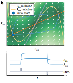
Reconstructing Computational System Dynamics Using RNNs

Figure1: State space and vector field of the Wilson–Cowan neural population model

In theory, the state space needs to be complete and unique to formally constitute a dynamical system (DS), as each point in the state space contains all information about the current state of the system and its future evolution. When starting from any specific initial condition, the system will move in the state space according to its vector field, thus producing a specific trajectory (trajectory or orbit). From a geometric perspective, each trajectory reflects the joint temporal evolution of system variables (e.g., firing rates of different neurons). The beauty of state space representation and its vector field lies in its ability to compactly and completely describe the behavior of DS, and the topological and geometric properties of the state space determine what computation the system performs.

To facilitate understanding of the representation of state space, we will introduce some geometric and topological concepts, including attractors, limit cycle attractors, chaotic attractors, and bifurcations.

The vector field of the neural model drives trajectories to converge to a specific point (referred to as a stable fixed point or stable equilibrium point in continuous time systems), and the neighborhood of convergence is referred to as their basin of attraction. Attractors can be single points or closed orbits, known as limit cycle attractors. Stable limit cycles correspond to nonlinear oscillations in the system, meaning that once the system’s state enters it, it continuously cycles along the closed orbit and is attracted to that orbit from some neighborhood of its basin of attraction. Limit cycles, like equilibrium points, can also be unstable or semi-stable, leading to deviations from the cycle even in one direction.

However, stable activity patterns in the nervous system do not necessarily need to be regular; just like in limit cycles, the system state may periodically return to all its previous positions; its activity patterns may also be highly irregular, which is referred to as chaotic attractors.

Another fundamental concept in DST that has significant implications for understanding physiology and computation is bifurcations.

Bifurcations refer to points or curves in parameter space where the topological structure of the system dynamics changes as the parameters vary smoothly. It is essential to note that parameters are distinct from the dynamical variables of the system; parameters are relatively stable characteristics of the system, often assumed to be constants. Parameters set the operating environment or conditions of the system, which are externally given and relatively stable; whereas variables represent the internal state of the system, dynamically changing as the system evolves. A key aspect of bifurcations is that when a critical point (bifurcation point) is crossed, the system dynamics can change dramatically. For instance, chaotic attractors may suddenly lose their stability.

DST in Neuroscience and RNN:

DST serves as a theoretical framework for understanding neural physiological functions and computation, with a long-standing tradition in neuroscience. For example, the pioneering work of Rinzel and Ermentrout and Izhikevich on the dynamical characterization of different spikes and burst behaviors in single cells used DST to understand large-scale network dynamics in neuronal populations and explore their connections to computation. However, these studies were based on “manual tuning” of biophysical models of neural systems, and constructing such models is a laborious and error-prone process.

RNNs were initially introduced as formal abstractions of neuronal systems for modeling time-varying processes. RNNs consist of a set of “neuronal” units that compute the weighted sum of their inputs and some nonlinear function changes. The difference between RNNs and the most commonly used feedforward neural networks (such as CNNs) is that RNNs allow for “reverberating” recurrent connections within the network. This feature also makes RNNs advantageous for simulating DS observed through experience.

Although DST is often used to analyze the dynamical mechanisms of RNNs trained for tasks, in this approach, neural or behavioral data obtained from animal experiments are not used as training data. In contrast, another advantage of RNNs is that they can be trained directly on neurophysiological data. RNNs trained on specific behavioral tasks are both convenient and powerful. For instance, the study by Yu et al. on neural trajectories in the motor cortex of macaques is one of the earliest examples. The RNN trained using this data extended the early studies of linear or generalized linear latent space models and allowed RNNs to infer and visualize smooth neural trajectories in low-dimensional state space by replacing linear latent models with nonlinear latent models.

Recently, generative models have gained popularity, and many people have encountered ambiguity in model classification. This article also mentions a conceptual misconception, where many people regard these data-inferred RNN models as generative models. After all, it is possible to sample new data from RNN models that statistically resemble the observed real data. However, this does not mean that data-inferred RNNs are generative in the DS sense—i.e., for the model to be generative in the dynamic systems sense—meaning the model can reproduce the long-term behavior of the underlying physiological system during simulation—this is a higher requirement. This requires that the model not only exhibits similar behavior within its training domain but also maintains this similarity outside the training domain, and can converge to the same attractor state as the real system, demonstrating the same vector field topology. To reliably ensure that this higher requirement is met, special training algorithms, optimization criteria, network architectures, and validation tests are typically necessary.

Reconstructing Trajectories from Time Series Data:

Next, we will explain how to reconstruct trajectories in time series. Generally, for a complex system like the brain, it may be challenging to establish a reliable mathematical model. However, if we start from the data, one might have a common question: can state space, trajectories, and their topological properties be inferred directly from experimental data?

A classic method for reconstructing trajectories directly from time series data is temporal delay embedding. We first assume that a time series scalar x obtained from the DS is available. Typically, x_t is obtained through some recording device. At time t, some function of the unknown DS state y is x=h(y(t)). The unknown state vector y that causes our observation may be some biophysical quantity, such as the membrane potentials of all neurons, or a more abstract quantity that thoroughly describes the potential DS. Based on the measurement x_t, by connecting the observed variables x at different lag times, we can form a time delay vector,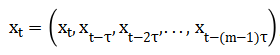 Reconstructing Computational System Dynamics Using RNNs , where m is the embedding dimension. The mechanism of forming these delayed embedding vectors from time series is called delay coordinate mapping.

One significant mathematical fact contained in the delay embedding theory is that if the embedding dimension m is sufficiently large, the trajectories reconstructed in the space of delayed coordinate vectors will represent the original trajectories in a 1:1 manner. In this case, all original topological properties will be preserved, resulting in the reconstructed state space. Here, topological preservation means that certain continuous deformations of the original state space are still allowed.

The delay embedding theorem provides important mathematical insights: in any empirical case, even with recordings from hundreds of neurons, it is impossible to ensure that all relevant dynamical variables are covered. The delay embedding theorem gives guidelines for augmenting the data space to ensure that dynamic objects in the reconstructed state space correspond topologically to those in the original DS. Importantly, dimensionality reduction tools commonly used to represent neural state spaces, such as principal component analysis (PCA), Isomap, or Laplacian eigenmaps, do not possess these properties and lack theoretical guarantees; dimensionality reduction may even destroy important dynamical characteristics. For example, PCA forms linear combinations of observations that may fail to distinguish between different states in the true state space of the DS or may distort its vector field.

To fully understand the computational processes being executed, access to the computational model of the DS is required. However, for delay coordinate maps, the computational model needs to adhere to certain topological requirements to faithfully represent the underlying dynamics. Only with such a model is it possible to study the detailed topology and geometry of attractors and vector fields.

Therefore, the key to DS reconstruction lies in how to infer the mathematical models of system dynamics directly from experimental data.

DS Reconstruction:

Since the dawn of science, humanity has utilized imagination and originality to infer natural laws through careful observation and experimental manipulation of the physical and biological worlds. However, establishing scientific models is a laborious, lengthy, and error-prone process. The flourishing development of ML and DL has provided us with the possibility to skip manual modeling. But we need to answer another question: can we infer the dynamical model of the system from observational data alone, such that its behavior in all aspects resembles that of the observed system?

The DL techniques used to achieve this goal are based on universal function approximators. Essentially, they are a set of powerful and expressive equations capable of approximating any other function to any desired precision.^{[NCC lab note 1]}

^{[NCC lab note]}Neural networks can fit arbitrary functions, as proven by the universal approximation theorem.

Thus, neural networks can be used to fit vector fields or any given DS trajectory. This process of approximation is referred to in machine learning as the training algorithm. The training algorithm is an iterative process used to adjust the parameters of the model system to approximate the target as closely as possible, such as minimizing the loss function, which means reducing the deviation between the current model output and the best-fitting data model output. However, most ordinary machine learning models do not possess universal approximation properties. For example, linear state space models fundamentally cannot produce most of the DS phenomena that interest us, such as limit cycles or chaos.

Another important point is that the mathematical form of the equations used for approximation may be entirely different from what human observers consider the most natural way to describe the real DS. For instance, “piecewise linear recurrent neural networks” (PLRNN) have been trained to approximate the DS of biophysical spiking neuron models. However, biophysical spiking neuron models are widely believed to be composed of differential equations that include exponential and polynomial terms, while PLRNNs themselves consist only of piecewise linear functions. Therefore, it is not necessary to have a detailed biological model specified by biophysical equations to perfectly simulate the dynamics of biological neurons. Theoretically, a set of universal neural networks or basis functions can reproduce any unknown DS with geometric and temporal characteristics, which is also the goal of DS reconstruction. Whether this theoretical ideal can be realized in practice largely depends on the training algorithm, and to a lesser extent on the network architecture used.

Training RNNs for DS Reconstruction:

In DS reconstruction, once trained on empirical data, these models will generate trajectories with topological and geometric structures in state space that correspond to the long-term temporal characteristics of the real DS. The most popular model for achieving this goal is RNN (as shown in Figure 2 process). Over the past few decades, various RNN architectures have existed, some representing discrete time, while others represent continuous time.

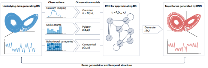
Reconstructing Computational System Dynamics Using RNNs

Figure 2: RNN-based dynamical system reconstruction

Many of these RNN architectures were designed to address certain practical problems encountered during training, the most prominent being the issues of “gradient vanishing” or “gradient explosion.” While in simple statistical models, such as linear regression, it is possible to analyze the optimal parameter solution in a single step, this is no longer feasible for most nonlinear models. Nonlinear network models typically use numerical gradient descent, such as the most famous backpropagation algorithm. These programs seek the optimal solution by sliding down the gradient of the loss function, iteratively moving the parameters toward the minimum of the loss. At this minimum, the model output is best aligned with the observed data.

Due to technical reasons, the loss gradient can rapidly decay or explode over long training sequences, the practical applicability of RNNs has been limited for quite some time. This has made it challenging to train RNNs on time series that may involve events occurring far apart in time, where event processes evolve very slowly, such as slow oscillations driven by rapid spikes (as shown in Figure 3)^{[NCC lab note 2]}^].

^{[NCC lab note 2]}^]In such cases, the limitation of not being able to learn long-term dependencies has been greatly alleviated in more modern transformer models; thus, many current time series models adopt transformer structures.

Reconstructing Computational System Dynamics Using RNNs

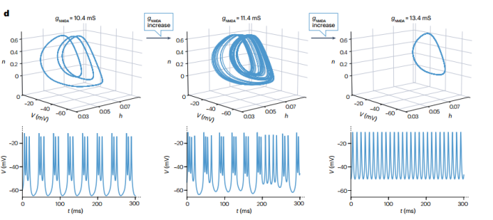
Figure 3: Slow oscillations driven by rapid spikes

Long Short-Term Memory (LSTM) networks were the first architecture to address this issue by integrating a protected “working memory” buffer, allowing the loss gradient to remain approximately constant (see Figure 4).

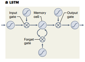
Reconstructing Computational System Dynamics Using RNNs

Figure 4: LSTM training process

Gated Recurrent Units (GRUs) are a simplified LSTM structure and have become widely adopted as an alternative to LSTMs. Recent architectures consider coupled or independent oscillators that can stably maintain information without bias. Another recent study aims to maintain the structural simplicity of the variants by applying specific constraints on parameters or by applying “soft constraints” in the loss function to gently push the parameters into a state of stable loss gradients during training, preventing uncontrollable loss gradient explosions.But the NCC lab would like to remind everyone that the DS reconstruction problem is actually different from classical machine learning problems. Scholars designing solutions for DS reconstruction often also consider classical machine learning applications, such as prediction or sequence-to-sequence regression; therefore, these architectures do not necessarily make RNNs more suitable for DS reconstruction. For chaotic systems, gradient explosion is theoretically unavoidable, as it results from trajectories that diverge exponentially in the system. Even in most complex biological or physical systems, chaotic dynamics are the norm rather than the exception.

Classification of DS Reconstruction Models::

To test the reconstruction capabilities of specific ML models or training algorithms, it is common to evaluate basic fact DS with known control equations first. By controlling gradient flow and other algorithmic techniques, RNNs such as LSTM (as shown in Figure 4) or PLRNN (as shown in Figure 2) can be trained to reconstruct complex chaotic, high-dimensional, or only partially observed DS. For example, after inferring appropriate initial conditions solely from data, RNNs can characterize the behavior of the real DS based on their control equations.

Reconstructing Computational System Dynamics Using RNNs

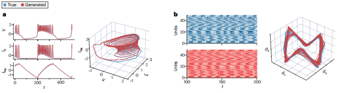
Figure 5: The explosion of a three-variable minimal biophysical NMDA-modulated bursting neuron model

Reservoir Computers and Echo State Machines are another clever RNN design that is popular in DS reconstruction, initially introduced as a computationally efficient alternative to classic RNNs. They consist of a large pool or “reservoir” of nonlinear units with fixed network connections. Training is performed only by adjusting the linear mapping of the reservoir to a layer of linear readout units fed back to the reservoir, thus providing the desired output for the network. Because the mappable reservoir is linear, the learning of these systems is very fast and is not affected by gradient explosion and vanishing issues. However, because they rely on a fixed large reservoir, it is not particularly clear whether they are genuinely performing DS reconstruction or merely predicting DS. Reservoir computers and echo state machines are also quite complex and high-dimensional, making them difficult to analyze as models of the underlying DS.

Most RNNs operate at discrete time steps but typically assume that the underlying DS evolves in continuous time and space. Therefore, continuous-time RNNs can better approximate the vector field of the observed DS, which is estimated through numerical differences along the observed time series using simple feedforward neural networks. This feedforward neural network is then reshaped into an RNN defined by differential equations. Neural Ordinary Differential Equations are essentially an extension of this idea, using deep feedforward neural networks reshaped into RNNs to approximate vector fields. Neural ordinary differential equations are a powerful tool for reconstructing observed DS in low dimensions and naturally extend to spatially continuous systems, such as dendrites. Due to their continuous time representation, neural ordinary differential equations can naturally handle observations that occur at irregular intervals, as they do not rely on discretizing time into equal binaries. Neural ordinary differential equations also easily allow the incorporation of prior domain knowledge in the form of known differential equations, such as in physics-based neural networks. However, as it stands, training neural ordinary differential equations seems to be more tedious, as they depend on numerical integration techniques to solve differential equations and loss gradients.

In contrast to RNNs, a more elegant idea is the sparse identification of nonlinear dynamical systems (SINDy), which uses a large basis function library to fit the observed DS, providing a degree of interpretability, as seen in Figure 6. SINDy is similar to LASSO regression, selecting a small number of functions from its large basis function library while forcing all other regression coefficients to be zero (L1 regularization to make it sparse). If the basis function library contains the correct terms that naturally describe the studied DS (e.g., if the DS equation consists of polynomial terms and the basis function library also contains the correct polynomials), SINDy is fast and highly accurate. However, if we cannot establish a suitable basis function library based on prior knowledge, SINDy often fails to converge to the correct solution. As in many empirical scenarios, we may not know the precise DS equations at all.

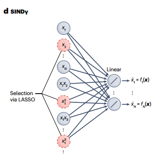
Reconstructing Computational System Dynamics Using RNNs

Figure 6: Sparse identification of nonlinear dynamical systems (SINDy)

Enhancing RNN Performance with Autoencoders:

Typically, the interest lies in facilitating DS learning and interpretability with the lowest dimensional dynamical representation or appropriate coordinate transformations. This can be achieved by embedding SINDy or any RNN into an autoencoder architecture (as shown in Figure 7). An autoencoder consists of a deep encoder and a deep decoder. The encoder network typically projects the observed data into a much lower-dimensional latent space configured to possess certain desired properties, and then the decoder recovers the original data from the latent representation. By combining this autoencoder with the DS reconstruction model and jointly training using a combined loss function, a latent model most suited for learning potential dynamics can be constructed.

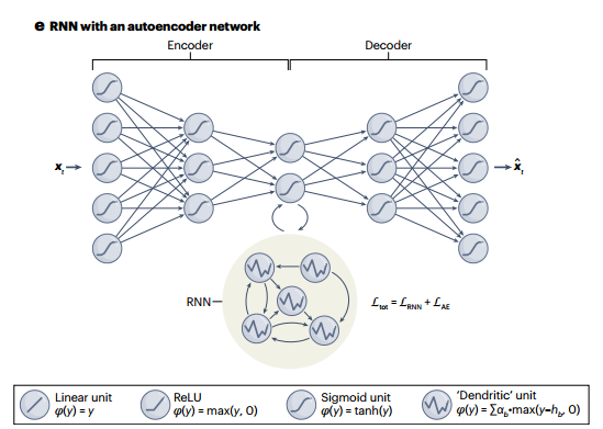
Reconstructing Computational System Dynamics Using RNNs

Figure 7: Embedding models into autoencoder architecture

Probabilistic RNN Formulations::

Some of the currently most successful DS reconstruction training methods (such as BPTT) assume that the latent model is deterministic; however, it is often more natural to assume that the latent dynamic process is stochastic. In fact, both discrete-time and continuous-time RNNs are equipped with probabilistic assumptions. Incorporating this stochasticity into the latent model requires special training and inference methods, which typically rely on what is known as the state space framework and expectation-maximization algorithms or variational inference techniques and variational autoencoders (VAEs).

This latent model provides a means for generating a holistic probability distribution of potential state spaces and parameters. Probabilistic DS reconstruction models also naturally explain various statistically recorded but different data patterns simultaneously. For example, neuroscience experiments may involve Poisson-type spike count data from many neurons. By connecting RNNs to different modality-specific decoder models, these models can be integrated into the same latent DS model, capturing the unique statistical characteristics of the three distinct data modalities observed. This establishes direct connections between different data patterns within a shared latent space, which can reveal relationships between neural trajectories, DS objects, and behavioral choice processes.

Evaluating Dynamical System Reconstruction::

How can we evaluate whether DS reconstruction is effective as expected? In ML, RNNs are primarily used for predicting the studied system in advance. For example, predicting power consumption or weather forecasting. Therefore, Mean Squared Prediction Error (MSPE) is commonly used to assess the performance of RNN training algorithms. However, MSPE is not applicable for evaluating DS reconstruction algorithms. Because if the underlying DS is chaotic, even if observations are extracted from precisely the same underlying DS, slight noise or differences in initial conditions can quickly lead to large MSPE, and vice versa. Therefore, relatively low MSPE may falsely indicate a high degree of fit between the real DS and the reconstructed DS, even though the underlying dynamics of these two systems may differ significantly.

Thus, in DS reconstruction, it is crucial to maintain the geometric properties and other time-invariant characteristics of the DS. For example, Kullback–Leibler divergence, Wasserstein distance, and Hellinger distance have been used to evaluate the geometric overlap of data point distributions between the invariant sets generated by the real DS and the reconstructed DS over large time scales. The maximum Lyapunov exponent, or the so-called correlation dimension (empirical estimate of the fractal dimension of attractors), is another example of such invariant dynamical and geometric DS properties. The consistency of the invariant temporal structures of real trajectories and reconstructed trajectories—i.e., the nature of temporal behavior, in the limit, does not depend on when measurements are taken—can be evaluated through the overlap of autocovariance functions or power spectra. Only when the reconstructed DS closely aligns with the data of these invariant geometric and temporal characteristics can it be further analyzed and interpreted as a potential model of the underlying system dynamics.

Analysis and Interpretation of RNNs::

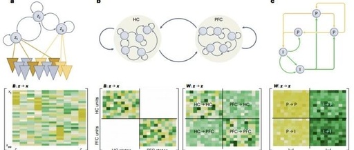
The RNN models trained on DS data (hereafter referred to as latent RNNs) can provide two different levels of interpretability:

First, the parameters of latent RNNs reflect certain physiological or anatomical characteristics of the latent DS, such as connectivity between neurons or brain regions (as shown in Figure 8).

Second, latent RNNs serve as substitutes for the dynamical processes of data generation, providing unprecedented interpretability and insights into the underlying computational mechanisms: DST tools can be used to reveal the internal workings of the model in detail.

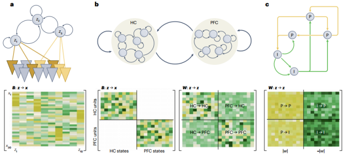
Reconstructing Computational System Dynamics Using RNNs

Figure 8: Evaluating connectivity between neurons or brain regions using RNNs

In the DS reconstruction process, there are numerous possibilities for endowing RNNs with direct physiological and anatomical interpretability. Typically, latent RNNs couple with actual measured neural or behavioral time series. If a generalized linear model form is adopted, connecting the latent RNN to the decoder model of the measurement data, the entries in the factor weight matrix B of the generalized linear model can be interpreted directly, as described in conventional or Gaussian process factor analysis. The entries in B reflect the joint loading of different observables on the same latent RNN state. For example, a set of units with large coefficients on the same latent state is active within the same unit component. If measurements are taken simultaneously from different data patterns, B can also determine the relationships between different patterns.

An interesting option is to constrain the structure of B: it can be constrained so that only a subset of the latent RNN states maps to a specific subset of observations, which can assign specific semantic roles, such as the roles of prefrontal neurons or pyramidal cells, to defined subsets of latent states. For instance, given recordings from different brain regions or cortices, B can be constrained so that only a subset of latent RNN states connects to one brain region, while different subsets of RNN states connect to a second brain region. Thus, the entries in the connectivity matrix W of the RNN will automatically be interpreted based on the strengths of connections within and between regions. As another example, suppose the recorded units can be divided into different categories, such as pyramidal cells and interneurons. By assigning subsets of latent states exclusively to one class or another and forcing their output weights to be only positive or negative, W will yield information about excitatory and inhibitory microcircuits and connectivity motifs.

When RNN reconstruction models are used as a conceptual framework to analyze the neural computations underlying cognitive and behavioral processes, they can become particularly powerful. The literature has proposed different hypotheses regarding the neural computational realization of working memory, such as multistability or slow approaches to bifurcation dynamics in the absence of stable states. Such hypotheses can now be directly tested by examining the vector fields and attractor objects of the trained RNN-based reconstruction models. We have the opportunity to uncover previously undiscovered dynamical mechanisms.

However, the analysis of DS largely depends on the dynamical accessibility and interpretability of the ML–AI models. If the mathematical setup of the RNNs used is relatively complex, such as in LSTMs or neural ordinary differential equations, approximate numerical methods will be needed to find the dynamical objects and structures of interest. Thus, many ideas that make ML–AI models interpretable in the DS sense are based on some form of local linear dynamics, as linear models are easier to handle, understand, and analyze. However, from a global perspective, a suitable DS model still needs to be nonlinear; otherwise, it will not produce phenomena such as limit cycles or chaos. Further enhancing interpretability can be achieved by discovering low-dimensional DS representations, for example, by improving the expressiveness of individual network units or jointly training with autoencoders to extract low-dimensional DS. Equally important are the analytical tools that connect the structure and dynamics of RNNs to computational and task performance; computational neuroscience has made significant progress in this area in recent years. Therefore, a particular challenge in the field of DS reconstruction is to design simple yet mathematically manageable models with strong expressive power.

Future Extensions

This article also presents the problems that need to be addressed and the directions that need to be tackled in this field:

1. First, the nervous system is highly dimensional. Modern neural recording technologies typically provide hundreds or thousands of simultaneous time series observations. Even so, this still represents only a small portion of all the dynamical variables in the biological substrate, for example, there are billions of neurons in a tiny mouse brain, not to mention all the cellular and molecular processes in the human brain. It cannot be ensured that all dynamically relevant variables are observed. How to infer the multi-scale dynamical system of the complete brain from different scales of partially observed neural data is a direction that needs to be tackled in the future.

2. Moreover, neural recording technologies often only represent block signals that need to be processed, usually providing filtered versions of the variables of interest or producing variables that may be highly non-Gaussian or even discontinuous. Even in principle, it is unclear how much detailed information about the potential dynamics can be retrieved from such observational data. We cannot determine to what extent different types of data preprocessing weaken or enhance the effectiveness of DS reconstruction.

3. Another significant challenge faced by DS reconstruction algorithms is that neuroscience data is often non-stationary and the observation process injects extra noise. Slow changes in the subject’s physical, motivational, or emotional states can affect the collection of neural data. The slow drift of parameters in the nervous system often leads to various types of complex bifurcations. Therefore, how to control or eliminate this additional complexity (non-stationary, bifurcations caused by noisy data) in DS reconstruction is an important research direction.

[Discussion in NCC lab]:

The friends in the NCC lab believe that data-driven DS reconstruction (especially RNN-based DS reconstruction) is still in its infancy. While this article showcases some training algorithms for DS reconstruction, thus far, many training algorithms for DS reconstruction have primarily been tested on relatively small benchmark systems, with little (if any) consideration for random observational noise, and assuming complete access to all system variables, large sample sizes, and stationary conditions. This sharply contrasts with the reality of neuroscience.

This article also proposes some solutions, such as explicitly designing DS reconstruction methods that map processes across multiple time scales may be helpful, but the choice of variables often only holds significance for specific variables. For example, there are many strong nonlinearities and higher-order characteristics in the nervous system, and heterogeneity of biophysics and synapses can easily lead to highly chaotic activity. Point attractors are often the result of averaging over faster time scales that dominate those based on chaos in many RNN-based analyses, but the latter may also be computationally relevant.

More generally, to date, most DS descriptions in neuroscience have focused on very simple DS objects, such as linear attractors or limit cycles. As different time and spatial scales are traversed, and as neuroscience continues to delve into more complex behaviors and decision-making in natural environments, there is a need to introduce more advanced DS theories and tools, including modeling of the direct problem of dynamical systems, solving inverse problems, evaluating reconstruction performance, controlling dynamical systems, and so on.

The neural dynamical models obtained through DS reconstruction can not only utilize modern powerful ML/AI methods for data fitting and system identification but can also conceptually integrate representations of neural dynamics, latent states, and observational behaviors across different spatiotemporal scales within neural computational theory. The potential brought about by data-driven DS reconstruction, along with the rich analytical tools provided by DST, may one day change our understanding of brain functions.

References

[1] Durstewitz, Daniel, Georgia Koppe, and Max Ingo Thurm. “Reconstructing computational system dynamics from neural data with recurrent neural networks.” Nature Reviews Neuroscience 24.11 (2023): 693-710.

[2] Rinzel, J. & Ermentrout, G. B. in Methods of Neuronal Modeling: From Synapses to Networks (eds Koch, C. & Segev, I.) 251–292 (MIT Press, 1998).

[3] Izhikevich, E. M. Dynamical Systems in Neuroscience (MIT Press, 2007).

[4] Yu, B. M. et al. Extracting dynamical structure embedded in neural activity. In Proc. 18th Advances in Neural Information Processing Systems (eds. Weiss, Y., Schölkopf, B. & Platt, J.) 1545-1552 (MIT Press, Vancouver, 2005).

[5] Kramer, D., Bommer, P. L., Tombolini, C., Koppe, G. & Durstewitz, D. Reconstructing nonlinear dynamical systems from multi-modal time series. In Proc. 39th International Conference on Machine Learning (eds Chaudhuri, K. et al.) 11613–11633 (PMLR, 2022).

Written by: Li Zongsheng

Proofread by: Liu Quanying, Sun Weiting

(Students find it hard to write, welcome to reward the authors)

Leave a Comment Cancel reply