Principles and Implementation of Diffusion Models (Pytorch)

This article discusses the development, principles, and code practices of diffusion models.

The catalyst for diffusion models began with the introduction of DDPM (Denoising Diffusion Probabilistic Model) in 2020. Before delving into the details of how the Denoising Diffusion Probabilistic Model (DDPM) works, let’s first look at some developments in existing generative artificial intelligence, which are the foundational studies of DDPM:

VAE

VAEs use encoders, probabilistic latent spaces, and decoders. During training, the encoder predicts the mean and variance for each image. These values are then sampled from a Gaussian distribution and passed to the decoder, where the input image is expected to resemble the output image. This process involves using KL Divergence to compute the loss. One significant advantage of VAEs is their ability to generate a wide variety of images. During the sampling phase, simply sampling from the Gaussian distribution allows the decoder to create a new image.

GAN

Shortly after the introduction of Variational Autoencoders (VAEs), a groundbreaking generative family of models emerged—Generative Adversarial Networks (GANs), marking the beginning of a new class of generative models characterized by the collaboration of two neural networks: a generator and a discriminator, involving an adversarial training process. The generator aims to produce realistic data, such as images, from random noise, while the discriminator strives to distinguish between real and generated data. Throughout the training phase, the generator and discriminator continuously refine their abilities through a competitive learning process. The generator generates increasingly convincing data, becoming smarter than the discriminator, while the discriminator improves its ability to discern real samples from generated ones. This adversarial interaction peaks when the generator produces high-quality, realistic data. During the sampling phase, after GAN training, the generator produces new samples from input random noise, transforming this noise into data that typically reflects real examples.

Why We Need Diffusion Models: DDPM

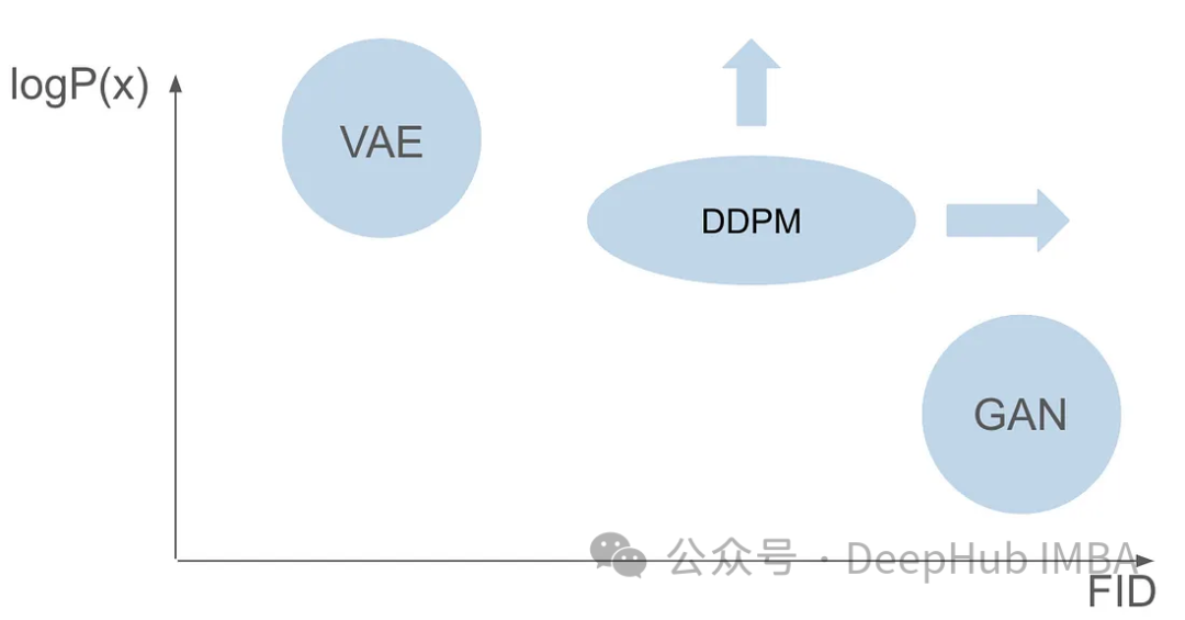
Both models have different issues; while GANs excel at generating realistic images that closely resemble those in the training set, VAEs are adept at creating a diverse array of images, although they tend to produce blurry images. However, existing models have not successfully combined these two capabilities—creating images that are both highly realistic and diverse. This challenge presents a significant barrier that researchers need to address.

Six years after the first GAN paper was published and seven years after the VAE paper, a groundbreaking model emerged: the Denoising Diffusion Probabilistic Model (DDPM). DDPM combines the advantages of both models, excelling at creating diverse and realistic images.

In this article, we will delve into the complexities of DDPM, covering its training process, including forward and reverse processes, and exploring how to perform sampling. Throughout this exploration, we will use PyTorch to build DDPM from scratch and complete its full training.

It is assumed that you are already familiar with the basics of deep learning and have a solid foundation in deep computer vision. We will not introduce these basic concepts; our goal is to generate images that humans believe to be real.

Diffusion Model DDPM

The Denoising Diffusion Probabilistic Model (DDPM) is a cutting-edge approach in the field of generative models. Unlike traditional models that rely on explicit likelihood functions, DDPM operates by iteratively denoising through the diffusion process. This involves gradually adding noise to an image and attempting to remove that noise. The fundamental theory is based on the idea that by transforming a simple distribution, such as a Gaussian distribution, through a series of diffusion steps, a complex and expressive image data distribution can be obtained. In other words, by transferring samples from the original image distribution to a Gaussian distribution, we can create a model that reverses this process. This allows us to start from a fully Gaussian distribution and end with an image distribution, effectively generating new images.

The training of DDPM involves two fundamental steps: generating noisy images, which is a fixed and non-learnable forward process, and the subsequent reverse process. The main goal of the reverse process is to denoise the images using a specialized machine learning model.

Forward Diffusion Process

The forward process is a fixed and non-learnable step, but it requires some predefined settings. Before delving into these settings, let’s understand how it works.

The core concept of this process is to start with a clear image. At a specific step denoted by “T”, a small amount of noise is gradually introduced according to a Gaussian distribution.

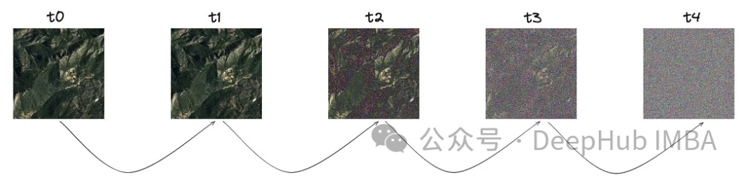
It can be seen from the image that noise is incrementally added at each step, and we will delve into the mathematical representation of this noise.

The noise is sampled from a Gaussian distribution. To introduce a small amount of noise at each step, we use a Markov chain. To generate the image at the current timestamp, we only need the image from the last timestamp. The concept of the Markov chain is key here and is crucial for the subsequent mathematical details.

A Markov chain is a stochastic process where the probability of transitioning to any specific state depends only on the current state and the time elapsed, rather than the sequence of previous events. This property simplifies the modeling of the noise addition process, making it easier for mathematical analysis.

The variance parameter denoted by beta is intentionally set to a very small value, with the aim of introducing only a minimal amount of noise at each step.

The step parameter “T” determines the number of steps required to generate a fully noisy image. In this article, this parameter is set to 1000, which may seem large. Do we really need to create 1000 noisy images for each original image in the dataset? The Markov chain aspect proves helpful in addressing this issue. Since we only need the image from the previous step to predict the next step, and the noise added at each step remains constant, we can simplify the calculations by generating noisy images at specific timestamps. The right reparameterization technique allows us to further simplify the equations.

The new parameters introduced in equation (3) are incorporated into equation (2), resulting in an evolution of equation (2).

Reverse Diffusion Process

Having introduced noise to the images, the next step is to perform the reverse operation. Mathematically, it is impossible to achieve reverse processing of the image unless we know the initial condition, namely the denoised image at t = 0. Our goal is to directly sample from noise to create new images, where there is a lack of information about the results. Therefore, I need to design a method to gradually denoise the image without knowing the results. Hence, the solution involves using a deep learning model to approximate this complex mathematical function.

With some mathematical background, the model will approximate equation (5). A noteworthy detail is that we will stick to the original DDPM paper and keep the variance fixed, although it is also possible to let the model learn it.

The task of the model is to predict the average noise added between the current timestamp and the previous timestamp. Doing so effectively removes noise and achieves the desired effect. However, what if our goal is to have the model predict the noise added from the “original image” to the last timestamp?

Mathematically, executing the reverse process is challenging unless we know the initial image without noise, so let’s start by defining the posterior variance.

The task of the model is to predict the noise added to the image at timestamp t from the initial image. The forward process enables us to perform this operation, starting from a clear image and progressing to a noisy image at timestamp t.

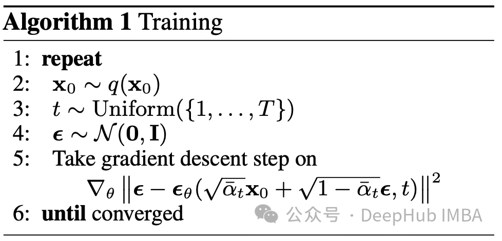
Training Algorithm

We assume that the architecture used for prediction will be a U-Net. The objective during the training phase is: for each image in the dataset, randomly select a timestamp in the range [0,T] and calculate the forward diffusion process. This generates a clear, slightly noisy image, along with the actual noise used. Then, utilizing our understanding of the reverse process, we use the model to predict the noise added to the image. With the real and predicted noise, we seem to have entered a supervised machine learning problem.

The main question arises: which loss function should we use to train our model? Since we are dealing with a probabilistic latent space, Kullback-Leibler (KL) divergence is a suitable choice.

KL divergence measures the difference between two probability distributions, in our case, the distribution predicted by the model and the expected distribution. Including KL divergence in the loss function not only guides the model to produce accurate predictions but also ensures that the latent space representation conforms to the expected probabilistic structure.

KL divergence can be approximated as an L2 loss function, so we can obtain the following loss function:

Ultimately, we arrive at the training algorithm proposed in the paper.

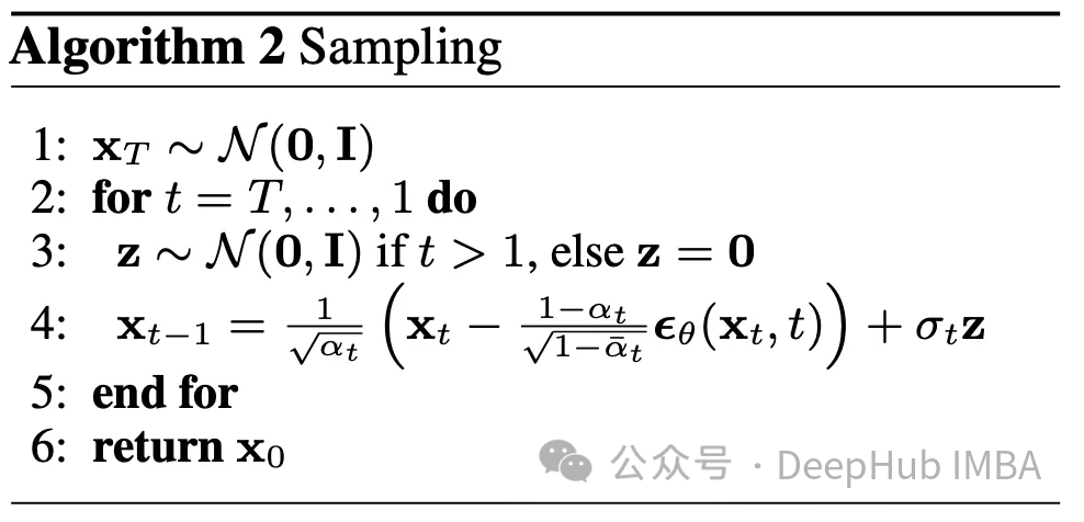
Sampling

The reverse process has been explained; now let’s discuss how to use it. Starting from a completely random image at time T and using the reverse process T times, we ultimately reach time 0. This constitutes the second algorithm outlined in this article.

Parameters

We have many different parameters such as beta, beta_tildes, alpha, alpha_hat, etc. Currently, we do not know how to choose these parameters. However, the only known parameter at this time is T, which is set to 1000.

For all listed parameters, their selection depends on beta. In a sense, beta determines the amount of noise we want to add at each step. Therefore, careful selection of beta is crucial to ensure the success of the algorithm. For the other parameters, please refer to the paper for details.

Various sampling methods were explored during the experimental phase of the original paper. The initial linear sampling methods either led to insufficient noise or became overly noisy. To address this issue, another more commonly used method, cosine sampling, was adopted. Cosine sampling provides smoother and more consistent noise addition.

Pytorch Implementation of Diffusion Models

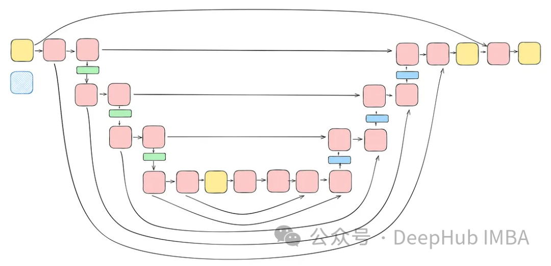
We will utilize the U-Net architecture for noise prediction. The choice of U-Net is due to its suitability for image processing, capturing spatial and feature maps, and providing output of the same size as the input.

Given the complexity of the task and the requirement to use the same model for each step (where the model needs to be able to denoise both completely noisy images and slightly noisy images with the same weights), adjusting the model is essential. This includes merging more complex blocks and introducing awareness of the timestamps used through sinusoidal embedding steps. These enhancements aim to make the model an expert in the denoising task. Before continuing to build the complete model, we will introduce each block.

ConvNext Block

To meet the need for increased model complexity, convolutional blocks play a crucial role. Here, we cannot solely rely on the basic blocks from the U-Net paper; we will incorporate ConvNext.

The input consists of “x” representing the image and a timestamp visualization “t” of size “time_embedding_dim”. Due to the complexity of the blocks and the residual connections with the input and final layer, the blocks play a key role in learning spatial and feature mapping throughout the process.

class ConvNextBlock(nn.Module): def __init__( self, in_channels, out_channels, mult=2, time_embedding_dim=None, norm=True, group=8, ): super().__init__() self.mlp = ( nn.Sequential(nn.GELU(), nn.Linear(time_embedding_dim, in_channels)) if time_embedding_dim else None ) self.in_conv = nn.Conv2d( in_channels, in_channels, 7, padding=3, groups=in_channels ) self.block = nn.Sequential( nn.GroupNorm(1, in_channels) if norm else nn.Identity(), nn.Conv2d(in_channels, out_channels * mult, 3, padding=1), nn.GELU(), nn.GroupNorm(1, out_channels * mult), nn.Conv2d(out_channels * mult, out_channels, 3, padding=1), ) self.residual_conv = ( nn.Conv2d(in_channels, out_channels, 1) if in_channels != out_channels else nn.Identity() ) def forward(self, x, time_embedding=None): h = self.in_conv(x) if self.mlp is not None and time_embedding is not None: assert self.mlp is not None, “MLP is None” h = h + rearrange(self.mlp(time_embedding), “b c -> b c 1 1”) h = self.block(h) return h + self.residual_conv(x)

Sinusoidal Timestamp Embedding

One of the key blocks in the model is the sinusoidal timestamp embedding block, which allows the encoding of a given timestamp to retain information about the current time needed for the model’s decoding, as it will be used for all different timestamps.

This is a very classic implementation and is applied in various places, so we will directly paste the code here.

class SinusoidalPosEmb(nn.Module): def __init__(self, dim, theta=10000): super().__init__() self.dim = dim self.theta = theta def forward(self, x): device = x.device half_dim = self.dim // 2 emb = math.log(self.theta) / (half_dim – 1) emb = torch.exp(torch.arange(half_dim, device=device) * -emb) emb = x[:, None] * emb[None, :] emb = torch.cat((emb.sin(), emb.cos()), dim=-1) return emb

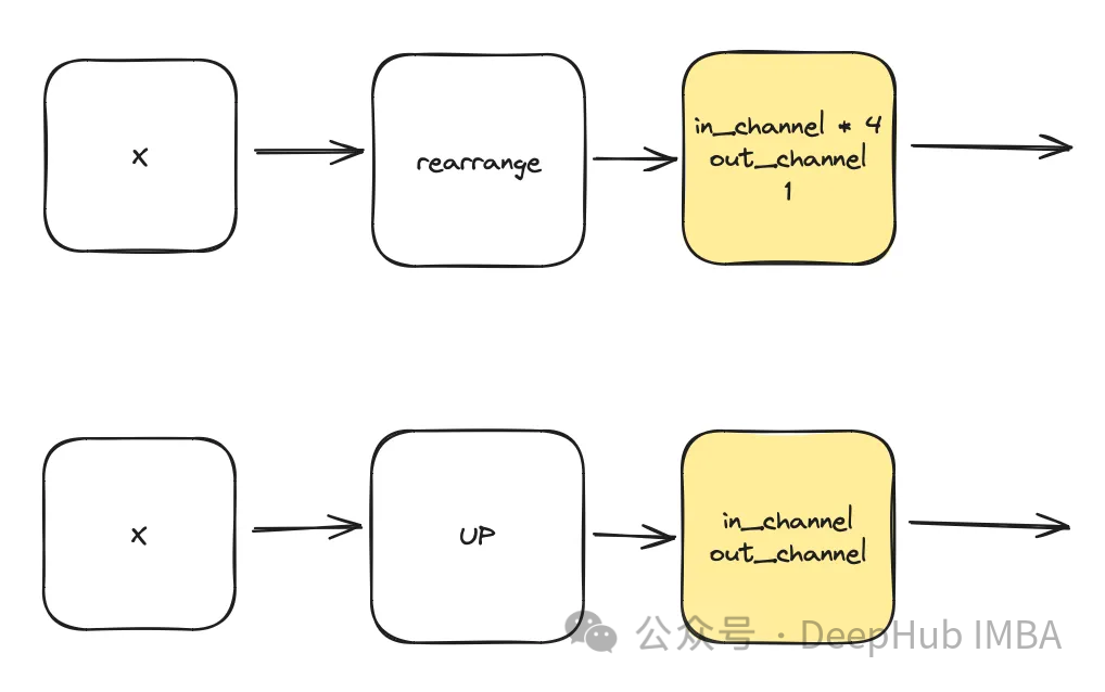
DownSample & UpSample

class DownSample(nn.Module): def __init__(self, dim, dim_out=None): super().__init__() self.net = nn.Sequential( Rearrange(“b c (h p1) (w p2) -> b (c p1 p2) h w”, p1=2, p2=2), nn.Conv2d(dim * 4, default(dim_out, dim), 1), ) def forward(self, x): return self.net(x) class Upsample(nn.Module): def __init__(self, dim, dim_out=None): super().__init__() self.net = nn.Sequential( nn.Upsample(scale_factor=2, mode=”nearest”), nn.Conv2d(dim, dim_out or dim, kernel_size=3, padding=1), ) def forward(self, x): return self.net(x)

Temporal Multilayer Perceptron

This module is utilized to create temporal representations based on the given timestamp t. The output of this multilayer perceptron (MLP) will also serve as the input “t” for all modified ConvNext blocks.

Here, “dim” is a hyperparameter of the model that indicates the number of channels required for the first block. It serves as the basis for calculating the number of channels in subsequent blocks.

sinu_pos_emb = SinusoidalPosEmb(dim, theta=10000) time_dim = dim * 4 time_mlp = nn.Sequential( sinu_pos_emb, nn.Linear(dim, time_dim), nn.GELU(), nn.Linear(time_dim, time_dim), )

Attention

This is an optional component used in U-Net. Attention helps enhance the role of residual connections in learning. It focuses more on important spatial information obtained from the left side of U-Net through the attention mechanism computed via the residual connections and the feature maps calculated in the mid-low latent space. It originates from the ACC-UNet paper.

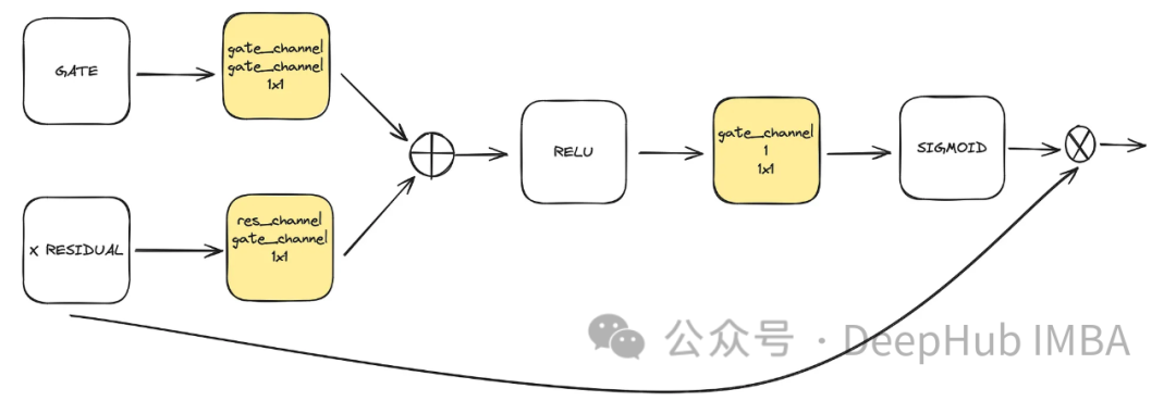
The gate represents the upsample output of the lower block, while the residual denotes the residual connection at the level where attention is applied.

class BlockAttention(nn.Module): def __init__(self, gate_in_channel, residual_in_channel, scale_factor): super().__init__() self.gate_conv = nn.Conv2d(gate_in_channel, gate_in_channel, kernel_size=1, stride=1) self.residual_conv = nn.Conv2d(residual_in_channel, gate_in_channel, kernel_size=1, stride=1) self.in_conv = nn.Conv2d(gate_in_channel, 1, kernel_size=1, stride=1) self.relu = nn.ReLU() self.sigmoid = nn.Sigmoid() def forward(self, x: torch.Tensor, g: torch.Tensor) -> torch.Tensor: in_attention = self.relu(self.gate_conv(g) + self.residual_conv(x)) in_attention = self.in_conv(in_attention) in_attention = self.sigmoid(in_attention) return in_attention * x

Final Integration

Integrate all the blocks discussed earlier (excluding the attention block) into a Unet. Each block contains two residual connections instead of one. This modification is made to address potential overfitting issues.

class TwoResUNet(nn.Module): def __init__( self, dim, init_dim=None, out_dim=None, dim_mults=(1, 2, 4, 8), channels=3, sinusoidal_pos_emb_theta=10000, convnext_block_groups=8, ): super().__init__() self.channels = channels input_channels = channels self.init_dim = default(init_dim, dim) self.init_conv = nn.Conv2d(input_channels, self.init_dim, 7, padding=3) dims = [self.init_dim, *map(lambda m: dim * m, dim_mults)] in_out = list(zip(dims[:-1], dims[1:])) sinu_pos_emb = SinusoidalPosEmb(dim, theta=sinusoidal_pos_emb_theta) time_dim = dim * 4 self.time_mlp = nn.Sequential( sinu_pos_emb, nn.Linear(dim, time_dim), nn.GELU(), nn.Linear(time_dim, time_dim), ) self.downs = nn.ModuleList([]) self.ups = nn.ModuleList([]) num_resolutions = len(in_out) for ind, (dim_in, dim_out) in enumerate(in_out): is_last = ind >= (num_resolutions – 1) self.downs.append( nn.ModuleList( [ ConvNextBlock( in_channels=dim_in, out_channels=dim_in, time_embedding_dim=time_dim, group=convnext_block_groups, ), ConvNextBlock( in_channels=dim_in, out_channels=dim_in, time_embedding_dim=time_dim, group=convnext_block_groups, ), DownSample(dim_in, dim_out) if not is_last else nn.Conv2d(dim_in, dim_out, 3, padding=1), ] ) ) mid_dim = dims[-1] self.mid_block1 = ConvNextBlock(mid_dim, mid_dim, time_embedding_dim=time_dim) self.mid_block2 = ConvNextBlock(mid_dim, mid_dim, time_embedding_dim=time_dim) for ind, (dim_in, dim_out) in enumerate(reversed(in_out)): is_last = ind == (len(in_out) – 1) is_first = ind == 0 self.ups.append( nn.ModuleList( [ ConvNextBlock( in_channels=dim_out + dim_in, out_channels=dim_out, time_embedding_dim=time_dim, group=convnext_block_groups, ), ConvNextBlock( in_channels=dim_out + dim_in, out_channels=dim_out, time_embedding_dim=time_dim, group=convnext_block_groups, ), Upsample(dim_out, dim_in) if not is_last else nn.Conv2d(dim_out, dim_in, 3, padding=1) ] ) ) default_out_dim = channels self.out_dim = default(out_dim, default_out_dim) self.final_res_block = ConvNextBlock(dim * 2, dim, time_embedding_dim=time_dim) self.final_conv = nn.Conv2d(dim, self.out_dim, 1) def forward(self, x, time): b, _, h, w = x.shape x = self.init_conv(x) r = x.clone() t = self.time_mlp(time) unet_stack = [] for down1, down2, downsample in self.downs: x = down1(x, t) unet_stack.append(x) x = down2(x, t) unet_stack.append(x) x = downsample(x) x = self.mid_block1(x, t) x = self.mid_block2(x, t) for up1, up2, upsample in self.ups: x = torch.cat((x, unet_stack.pop()), dim=1) x = up1(x, t) x = torch.cat((x, unet_stack.pop()), dim=1) x = up2(x, t) x = upsample(x) x = torch.cat((x, r), dim=1) x = self.final_res_block(x, t) return self.final_conv(x)

Implementation of Diffusion Code

Finally, we introduce how diffusion is implemented. Since we have already covered all the mathematical theories used for the forward, reverse, and sampling processes, here we will focus on the code.

class DiffusionModel(nn.Module): SCHEDULER_MAPPING = { “linear”: linear_beta_schedule, “cosine”: cosine_beta_schedule, “sigmoid”: sigmoid_beta_schedule, } def __init__( self, model: nn.Module, image_size: int, *, beta_scheduler: str = “linear”, timesteps: int = 1000, schedule_fn_kwargs: dict | None = None, auto_normalize: bool = True, ) -> None: super().__init__() self.model = model self.channels = self.model.channels self.image_size = image_size self.beta_scheduler_fn = self.SCHEDULER_MAPPING.get(beta_scheduler) if self.beta_scheduler_fn is None: raise ValueError(f”unknown beta schedule {beta_scheduler}”) if schedule_fn_kwargs is None: schedule_fn_kwargs = {} betas = self.beta_scheduler_fn(timesteps, **schedule_fn_kwargs) alphas = 1.0 – betas alphas_cumprod = torch.cumprod(alphas, dim=0) alphas_cumprod_prev = F.pad(alphas_cumprod[:-1], (1, 0), value=1.0) posterior_variance = ( betas * (1.0 – alphas_cumprod_prev) / (1.0 – alphas_cumprod) ) register_buffer = lambda name, val: self.register_buffer( name, val.to(torch.float32) ) register_buffer(“betas”, betas) register_buffer(“alphas_cumprod”, alphas_cumprod) register_buffer(“alphas_cumprod_prev”, alphas_cumprod_prev) register_buffer(“sqrt_recip_alphas”, torch.sqrt(1.0 / alphas)) register_buffer(“sqrt_alphas_cumprod”, torch.sqrt(alphas_cumprod)) register_buffer( “sqrt_one_minus_alphas_cumprod”, torch.sqrt(1.0 – alphas_cumprod) ) register_buffer(“posterior_variance”, posterior_variance) timesteps, *_ = betas.shape self.num_timesteps = int(timesteps) self.sampling_timesteps = timesteps self.normalize = normalize_to_neg_one_to_one if auto_normalize else identity self.unnormalize = unnormalize_to_zero_to_one if auto_normalize else identity @torch.inference_mode() def p_sample(self, x: torch.Tensor, timestamp: int) -> torch.Tensor: b, *_, device = *x.shape, x.device batched_timestamps = torch.full( (b,), timestamp, device=device, dtype=torch.long ) preds = self.model(x, batched_timestamps) betas_t = extract(self.betas, batched_timestamps, x.shape) sqrt_recip_alphas_t = extract( self.sqrt_recip_alphas, batched_timestamps, x.shape ) sqrt_one_minus_alphas_cumprod_t = extract( self.sqrt_one_minus_alphas_cumprod, batched_timestamps, x.shape ) predicted_mean = sqrt_recip_alphas_t * ( x – betas_t * preds / sqrt_one_minus_alphas_cumprod_t ) if timestamp == 0: return predicted_mean else: posterior_variance = extract( self.posterior_variance, batched_timestamps, x.shape ) noise = torch.randn_like(x) return predicted_mean + torch.sqrt(posterior_variance) * noise @torch.inference_mode() def p_sample_loop( self, shape: tuple, return_all_timesteps: bool = False ) -> torch.Tensor: batch, device = shape[0], “mps” img = torch.randn(shape, device=device) # This cause me a RunTimeError on MPS device due to MPS back out of memory # No ideas how to resolve it at this point # imgs = [img] for t in tqdm(reversed(range(0, self.num_timesteps)), total=self.num_timesteps): img = self.p_sample(img, t) # imgs.append(img) ret = img # if not return_all_timesteps else torch.stack(imgs, dim=1) ret = self.unnormalize(ret) return ret def sample( self, batch_size: int = 16, return_all_timesteps: bool = False ) -> torch.Tensor: shape = (batch_size, self.channels, self.image_size, self.image_size) return self.p_sample_loop(shape, return_all_timesteps=return_all_timesteps) def q_sample( self, x_start: torch.Tensor, t: int, noise: torch.Tensor = None ) -> torch.Tensor: if noise is None: noise = torch.randn_like(x_start) sqrt_alphas_cumprod_t = extract(self.sqrt_alphas_cumprod, t, x_start.shape) sqrt_one_minus_alphas_cumprod_t = extract( self.sqrt_one_minus_alphas_cumprod, t, x_start.shape ) return sqrt_alphas_cumprod_t * x_start + sqrt_one_minus_alphas_cumprod_t * noise def p_loss( self, x_start: torch.Tensor, t: int, noise: torch.Tensor = None, loss_type: str = “l2”, ) -> torch.Tensor: if noise is None: noise = torch.randn_like(x_start) x_noised = self.q_sample(x_start, t, noise=noise) predicted_noise = self.model(x_noised, t) if loss_type == “l2”: loss = F.mse_loss(noise, predicted_noise) elif loss_type == “l1”: loss = F.l1_loss(noise, predicted_noise) else: raise ValueError(f”unknown loss type {loss_type}”) return loss def forward(self, x: torch.Tensor) -> torch.Tensor: b, c, h, w, device, img_size = *x.shape, x.device, self.image_size assert h == w == img_size, f”image size must be {img_size}” timestamp = torch.randint(0, self.num_timesteps, (1,)).long().to(device) x = self.normalize(x) return self.p_loss(x, timestamp)

The diffusion process is the training part of the model. It opens up a sampling interface that allows us to generate samples using the already trained model.

Summary of Training Points

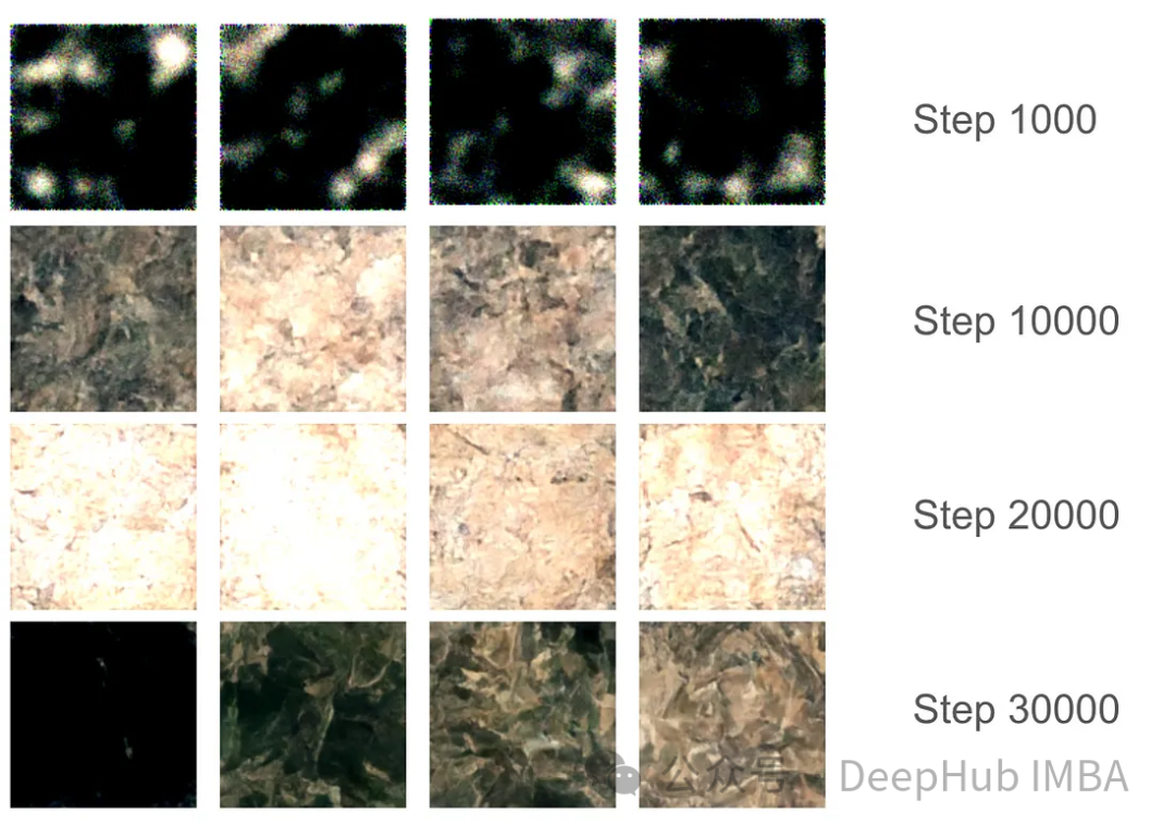
For the training part, we set up 37,000 training steps with a batch size of 16. Due to GPU memory allocation limits, the image size was restricted to 128×128. Using exponential moving average (EMA) model weights, samples were generated every 1000 steps to smooth sampling and save model versions.

In the initial 1000 training steps, the model began to capture some features but still missed certain areas. Around 10,000 steps, the model started producing promising results, and progress became more evident. By the final 30,000 steps, the quality of the results significantly improved, but black images still existed. This was simply due to the model not having enough sample variety, as the data distribution of real images was not fully mapped to the Gaussian distribution.

With the final model weights, we can generate some images. Although the image quality is limited due to the 128×128 size restriction, the model’s performance is still commendable.

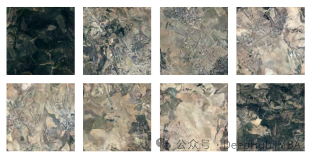
Note: The dataset used in this article consists of satellite images of forest terrains; for specific acquisition methods, please refer to the ETL section in the source code.

Conclusion

We have comprehensively introduced the necessary knowledge about diffusion models and provided a complete implementation using PyTorch.

Code for this article:

https://github.com/Camaltra/this-is-not-real-aerial-imagery/

Related papers:

DDPM Paper https://arxiv.org/abs/2006.11239ConvNext Paper https://arxiv.org/abs/2201.03545UNet Paper: https://arxiv.org/abs/1505.04597ACC UNet: https://arxiv.org/abs/2308.13680

Editor / Fan Ruiqiang

Review / Fan Ruiqiang

Verification / Fan Ruiqiang