

-
Overview -
Task Description -
Dataset -
Running Results -
Statistical Learning Methods -
Conditional Random Field (CRF) -
Deep Learning Methods -
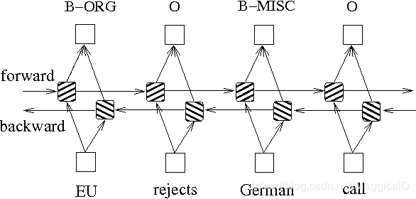
Bi-LSTM -
Bi-LSTM+CRF -
Points to Note in the Code
Overview
Task Description
Named Entity Recognition (English: Named Entity Recognition, abbreviated as NER) refers to identifying entities in text that have specific meanings, mainly including names of people, places, organizations, proper nouns, etc., as well as time, quantity, currency, ratio values, etc.
ACM announced that the three creators of deep learning, Yoshua Bengio, Yann LeCun, and Geoffrey Hinton, received the Turing Award in 2019.
-
Organization Name: ACM -
Person Name: Yoshua Bengio, Yann LeCun, Geoffrey Hinton -
Time: 2019 -
Proper Noun: Turing Award
Dataset
美  B-LOC国  E-LOC的  O华  B-PER莱  I-PER士  E-PER
我  O跟  O他  O谈  O笑  O风  O生  O
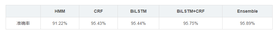
Running Results
Statistical Learning Methods
 , the probability of the next word’s label being
 is
is ),the observation probability matrix indicates the probability of generating a certain word under a specific label. Based on the three elements of HMM, we can define the following HMM model:
class HMM(object):    def __init__(self, N, M):        """Args:            N: Number of states, corresponding to the types of labels            M: Number of observations, corresponding to the number of different characters        """        self.N = N        self.M = M
        # State transition probability matrix A[i][j] indicates the probability of transitioning from state i to state j        self.A = torch.zeros(N, N)        # Observation probability matrix, B[i][j] indicates the probability of generating observation j under state i        self.B = torch.zeros(N, M)        # Initial state probability  Pi[i] indicates the probability of being in state i at the initial moment        self.Pi = torch.zeros(N)
<span>k/N</span>, which is quite simple, right? Using this method, we can approximate the three elements of HMM, as shown in the following code (functions that have appeared will be replaced with ellipses):class HMM(object): def __init__(self, N, M): .... def train(self, word_lists, tag_lists, word2id, tag2id): """Training HMM, estimating model parameters based on training corpus, because we have the observation sequence and its corresponding state sequence, we can use maximum likelihood estimation to estimate the parameters of the Hidden Markov Model. Args: word_lists: A list where each element is a list of characters, e.g., ['担','任','科','员'] tag_lists: A list where each element is a list of corresponding labels, e.g., ['O','O','B-TITLE', 'E-TITLE'] word2id: A mapping of characters to IDs tag2id: A dictionary mapping labels to IDs """ assert len(tag_lists) == len(word_lists)
# Estimate the transition probability matrix for tag_list in tag_lists: seq_len = len(tag_list) for i in range(seq_len - 1): current_tagid = tag2id[tag_list[i]] next_tagid = tag2id[tag_list[i+1]] self.A[current_tagid][next_tagid] += 1 # An important issue: if a certain element has never appeared, its position will be 0, which is not allowed in subsequent calculations. # Solution: We add a very small number to the probability that equals 0. self.A[self.A == 0.] = 1e-10 self.A = self.A / self.A.sum(dim=1, keepdim=True)
# Estimate the observation probability matrix for tag_list, word_list in zip(tag_lists, word_lists): assert len(tag_list) == len(word_list) for tag, word in zip(tag_list, word_list): tag_id = tag2id[tag] word_id = word2id[word] self.B[tag_id][word_id] += 1 self.B[self.B == 0.] = 1e-10 self.B = self.B / self.B.sum(dim=1, keepdim=True)
# Estimate the initial state probability for tag_list in tag_lists: init_tagid = tag2id[tag_list[0]] self.Pi[init_tagid] += 1 self.Pi[self.Pi == 0.] = 1e-10 self.Pi = self.Pi / self.Pi.sum()
class HMM(object):    ...    def decoding(self, word_list, word2id, tag2id):        """        Use the Viterbi algorithm to find the state sequence for the given observation sequence, here it is to find the corresponding labels for the sequence of characters.        The Viterbi algorithm actually uses dynamic programming to solve the prediction problem of the Hidden Markov Model, that is, using dynamic programming to find the maximum probability path (optimal path).        At this time, a path corresponds to a state sequence.        """        # Problem: In the case of a very long chain, multiplying many small probabilities may lead to underflow.        # Solution: Use log probabilities, so that very small probabilities in the source space are mapped to large negative numbers in the log space.        # Multiplication operations also become simple addition operations.        A = torch.log(self.A)        B = torch.log(self.B)        Pi = torch.log(self.Pi)
        # Initialize the Viterbi matrix viterbi, with dimensions [number of states, sequence length].        # Where viterbi[i, j] indicates the maximum probability of the j-th label being i in all single sequences (i_1, i_2, ..i_j).        seq_len = len(word_list)        viterbi = torch.zeros(self.N, seq_len)        # backpointer is a matrix of the same size as viterbi.        # backpointer[i, j] stores the id of the j-1-th label when the j-th label of the sequence is i.        # During decoding, we use backpointer to backtrack to find the optimal path.        backpointer = torch.zeros(self.N, seq_len).long()
        # self.Pi[i] indicates the probability of the first character being labeled as i.        # Bt[word_id] indicates the probability distribution of each label when the character is word_id.        # self.A.t()[tag_id] indicates the probability of transitioning from any state to the tag_id.
        # So the first step is        start_wordid = word2id.get(word_list[0], None)        Bt = B.t()        if start_wordid is None:            # If the character is not in the dictionary, assume the probability distribution of the states is uniform.            bt = torch.log(torch.ones(self.N) / self.N)        else:            bt = Bt[start_wordid]        viterbi[:, 0] = Pi + bt        backpointer[:, 0] = -1
        # Recursion formula:        # viterbi[tag_id, step] = max(viterbi[:, step-1]* self.A.t()[tag_id] * Bt[word])        # Where word is the character corresponding to the step time.        # Use the above recursion formula to find the subsequent steps.        for step in range(1, seq_len):            wordid = word2id.get(word_list[step], None)            # Handle cases where the character is not in the dictionary.            # bt is the probability distribution of the states when the character is wordid at time t.            if wordid is None:                # If the character is not in the dictionary, assume the probability distribution of the states is uniform.                bt = torch.log(torch.ones(self.N) / self.N)            else:                bt = Bt[wordid]  # Otherwise, take bt from the observation probability matrix.            for tag_id in range(len(tag2id)):                max_prob, max_id = torch.max(                    viterbi[:, step-1] + A[:, tag_id],                    dim=0                )                viterbi[tag_id, step] = max_prob + bt[tag_id]                backpointer[tag_id, step] = max_id
        # Termination, t=seq_len, the maximum probability in viterbi[:, seq_len] is the probability of the optimal path.        best_path_prob, best_path_pointer = torch.max(            viterbi[:, seq_len-1], dim=0        )
        # Backtrack to find the optimal path        best_path_pointer = best_path_pointer.item()        best_path = [best_path_pointer]        for back_step in range(seq_len-1, 0, -1):            best_path_pointer = backpointer[best_path_pointer, back_step]            best_path_pointer = best_path_pointer.item()            best_path.append(best_path_pointer)
        # Convert the sequence of tag_ids into tags.        assert len(best_path) == len(word_list)        id2tag = dict((id_, tag) for tag, id_ in tag2id.items())        tag_list = [id2tag[id_] for id_ in reversed(best_path)]        return tag_list
Conditional Random Field (CRF)
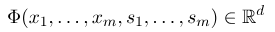
 indicates the observation sequence, and
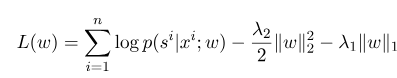
 indicates the state sequence. Then, the Conditional Random Field uses a log-linear model to calculate the conditional probability of the state sequence given the observation sequence:
 are:
are: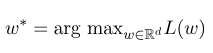
from sklearn_crfsuite import CRF   # The specific implementation of CRF is too complex, here we use an external library.

def word2features(sent, i):    """Extract features for a single character"""    word = sent[i]    prev_word = "<s>" if i == 0 else sent[i-1]    next_word = "</s>" if i == (len(sent)-1) else sent[i+1]    # Since the adjacent words will affect the label of this word, we use:    # Previous word, current word, next word,    # Previous word + current word, current word + next word    # as features    features = {        'w': word,        'w-1': prev_word,        'w+1': next_word,        'w-1:w': prev_word+word,        'w:w+1': word+next_word,        'bias': 1    }    return features

def sent2features(sent):    """Extract sequence features"""    return [word2features(sent, i) for i in range(len(sent))]

class CRFModel(object):    def __init__(self,                 algorithm='lbfgs',                 c1=0.1,                 c2=0.1,                 max_iterations=100,                 all_possible_transitions=False                 ):        self.model = CRF(algorithm=algorithm,                         c1=c1,                         c2=c2,                         max_iterations=max_iterations,                         all_possible_transitions=all_possible_transitions)
    def train(self, sentences, tag_lists):        """Train the model"""        features = [sent2features(s) for s in sentences]        self.model.fit(features, tag_lists)
    def test(self, sentences):        """Decode, predict the labels for the given sentences"""        features = [sent2features(s) for s in sentences]        pred_tag_lists = self.model.predict(features)        return pred_tag_lists
Deep Learning Methods
Bi-LSTM
import torchimport torch.nn as nnfrom torch.nn.utils.rnn import pad_packed_sequence, pack_padded_sequence

class BiLSTM(nn.Module):    def __init__(self, vocab_size, emb_size, hidden_size, out_size):        """Initialize parameters:            vocab_size: size of the dictionary            emb_size: dimension of the word vectors            hidden_size: dimension of the hidden vectors            out_size: number of labels        """        super(BiLSTM, self).__init__()        self.embedding = nn.Embedding(vocab_size, emb_size)        self.bilstm = nn.LSTM(emb_size, hidden_size,                              batch_first=True,                              bidirectional=True)
        self.lin = nn.Linear(2*hidden_size, out_size)
    def forward(self, sents_tensor, lengths):        emb = self.embedding(sents_tensor)  # [B, L, emb_size]
        packed = pack_padded_sequence(emb, lengths, batch_first=True)        rnn_out, _ = self.bilstm(packed)        # rnn_out:[B, L, hidden_size*2]        rnn_out, _ = pad_packed_sequence(rnn_out, batch_first=True)
        scores = self.lin(rnn_out)  # [B, L, out_size]
        return scores
    def test(self, sents_tensor, lengths, _):        """Decode"""        logits = self.forward(sents_tensor, lengths)  # [B, L, out_size]        _, batch_tagids = torch.max(logits, dim=2)
        return batch_tagid
Bi-LSTM+CRF
class BiLSTM_CRF(nn.Module): def __init__(self, vocab_size, emb_size, hidden_size, out_size): """Initialize parameters: vocab_size: size of the dictionary emb_size: dimension of the word vectors hidden_size: dimension of the hidden vectors out_size: number of labels """ super(BiLSTM_CRF, self).__init__() # Here, BiLSTM is the LSTM model part defined above. self.bilstm = BiLSTM(vocab_size, emb_size, hidden_size, out_size)
# CRF actually learns a transition matrix [out_size, out_size] initialized to a uniform distribution. self.transition = nn.Parameter( torch.ones(out_size, out_size) * 1/out_size) # self.transition.data.zero_()
def forward(self, sents_tensor, lengths): # [B, L, out_size] emission = self.bilstm(sents_tensor, lengths)
# Calculate CRF scores, this scores has size [B, L, out_size, out_size] # That is, each character corresponds to a [out_size, out_size] matrix # The element at the i-th row and j-th column of this matrix indicates: the score when the previous tag is i and the current tag is j. batch_size, max_len, out_size = emission.size() crf_scores = emission.unsqueeze( 2).expand(-1, -1, out_size, -1) + self.transition.unsqueeze(0)
return crf_scores
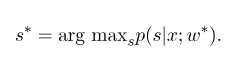
def test(self, test_sents_tensor, lengths, tag2id): """Use the Viterbi algorithm for decoding""" start_id = tag2id['<start>'] end_id = tag2id['<end>'] pad = tag2id['<pad>'] tagset_size = len(tag2id)
crf_scores = self.forward(test_sents_tensor, lengths) device = crf_scores.device # B:batch_size, L:max_len, T:target set size B, L, T, _ = crf_scores.size() # viterbi[i, j, k] indicates the maximum score of the k-th tag for the i-th sentence and the j-th character. viterbi = torch.zeros(B, L, T).to(device) # backpointer[i, j, k] indicates the id of the previous tag for the i-th sentence, the j-th character, and the k-th tag, used for backtracking. backpointer = (torch.zeros(B, L, T).long() * end_id).to(device) lengths = torch.LongTensor(lengths).to(device) # Forward recursion for step in range(L): batch_size_t = (lengths > step).sum().item() if step == 0: # The first character can only have start_id as its previous tag. viterbi[:batch_size_t, step, :] = crf_scores[: batch_size_t, step, start_id, :] backpointer[:batch_size_t, step, :] = start_id else: max_scores, prev_tags = torch.max( viterbi[:batch_size_t, step-1, :].unsqueeze(2) + crf_scores[:batch_size_t, step, :, :], # [B, T, T] dim=1 ) viterbi[:batch_size_t, step, :] = max_scores backpointer[:batch_size_t, step, :] = prev_tags
# During backtracking, we only need to use the backpointer matrix. backpointer = backpointer.view(B, -1) # [B, L * T] tagids = [] # Store results tags_t = None for step in range(L-1, 0, -1): batch_size_t = (lengths > step).sum().item() if step == L-1: index = torch.ones(batch_size_t).long() * (step * tagset_size) index = index.to(device) index += end_id else: prev_batch_size_t = len(tags_t) new_in_batch = torch.LongTensor( [end_id] * (batch_size_t - prev_batch_size_t)).to(device) offset = torch.cat( [tags_t, new_in_batch], dim=0 ) # This offset is actually the previous moment's index = torch.ones(batch_size_t).long() * (step * tagset_size) index = index.to(device) index += offset.long()
tags_t = backpointer[:batch_size_t].gather( dim=1, index=index.unsqueeze(1).long()) tags_t = tags_t.squeeze(1) tagids.append(tags_t.tolist())
# tagids:[L-1] (L-1 because the end_token is omitted), where each element in the list is the tag for that batch at that moment. # The following corrects its order and converts the dimension to [B, L]. tagids = list(zip_longest(*reversed(tagids), fillvalue=pad)) tagids = torch.Tensor(tagids).long()
# Return the decoding results return tagids
Points to Note in the Code
-
In the HMM model, it is necessary to handle the OOV (Out of Vocabulary) problem, where some characters in the test set are not in the training set. In this case, it is impossible to query the probabilities of various states corresponding to OOV through the observation probability matrix. To solve this problem, the probability distribution of the states corresponding to OOV can be set to a uniform distribution. -
During the estimation process of the three parameters of HMM (i.e., state transition probability matrix, observation probability matrix, and initial state probability matrix) using supervised learning methods, if some items have never appeared, the corresponding position will be 0. When using the Viterbi algorithm for decoding, if any of these values are 0, the probability of the entire path will also become 0. Additionally, during the decoding process, multiplying multiple small probabilities may lead to underflow. To address these two issues, we assign a very small number (e.g., 0.00000001) to those items that have never appeared, while also mapping the three parameters of the model to the log space during decoding. This avoids underflow and simplifies multiplication operations. -
In CRF, both training data and testing data must first extract features using feature functions before being input into the model! -
The Bi-LSTM+CRF model can refer to: Neural Architectures for Named Entity Recognition. Pay special attention to the definition of the loss function in it. The code for the calculation of the loss function uses a method similar to dynamic programming, which is not easy to understand. Here are some recommended blogs:
Important! The Yizhen Natural Language Processing Academic WeChat Group has been established.
You can scan the QR code below, and the assistant will invite you to join the group for communication.
Note: Please modify the remarks to [School/Company + Name + Direction] when adding.
For example — Harbin Institute of Technology + Zhang San + Dialogue System.
The account owner, please avoid business promotions. Thank you!


Recommended Reading:
The Difference and Connection Between Fully Connected Graph Convolutional Networks (GCN) and Self-Attention Mechanisms
Complete Guide for Beginners on Graph Convolutional Networks (GCN)

Paper Review [ACL18] Component Syntax Analysis Based on Self-Attentive