Source: PaperWeekly


This article is about 2300 words long, and it is recommended to read in 9 minutes.
This article mainly discusses solutions to the class imbalance problem, which can be divided into data-level resampling and model loss improvements.
The class imbalance issue in NLP tasks is indeed a very common and troublesome problem. Recently, I encountered this issue at work and spent some time sorting out and practicing solutions for class imbalance, mainly experimenting with “modified” loss functions (focal loss, GHM loss, dice loss, etc.), summarized as follows.
All the loss implementation codes can be found here:
https://github.com/shuxinyin/NLP-Loss-Pytorch
The data imbalance problem can also be referred to as a long-tail problem, where the long-tail portion of the data is often important and cannot be ignored. It is not just about the imbalance in the number of samples under classification labels; it is essentially also about the imbalance of easy and hard samples.
Solutions to the imbalance problem generally start from two aspects:
-
Data level: Resampling to ensure that the data participating in iterative calculations is balanced;
-
Model level: Reweighting to modify the model’s loss, increasing the loss reward for minority samples in the loss calculation.
Regarding data-level resampling, methods are generally through sampling to reconstruct the data distribution to achieve balance. There are three commonly used methods:
-
Under-sampling;
-
Over-sampling;
-
SMOTE.
1. Under-sampling: This refers to a category where there are many samples, so only part of the data is taken, directly discarding some data. This method is too simplistic and crude, resulting in a model with high bias and poor generalization performance;
2. Over-sampling: This method is the opposite of under-sampling; in categories with fewer samples, repeated sampling is performed to achieve data balance. The repeated calculations on these few samples can lead to overfitting of the model.
3. SMOTE: A type of neighbor interpolation that can reduce the risk of overfitting, but it is suitable for regression prediction scenarios, while NLP tasks are generally discrete.
Using these methods alone can lead to some waste or redundancy of data; they are generally combined with ensemble methods, sampling multiple sets of data, training multiple models, and then aggregating the results.
However, the above methods are often rarely used in engineering practice, partly because real data is precious and partly because the resource consumption of deploying ensemble methods is unacceptable. Therefore, we will focus on the reweighted loss improvements.
2. Model-Level Reweighting
Reweighting mainly refers to adjusting the contribution of class weights to the loss during the loss calculation phase. Classic loss improvements include Focal Loss, GHM Loss, and Dice Loss.
Focal Loss is a classic loss function designed to address imbalance issues, with the basic idea of focusing attention on samples that are predicted incorrectly.
What are incorrectly predicted samples? For example, positive samples with a predicted value less than 0.5, or negative samples with a predicted value greater than 0.5. Simply put, when the predicted value of a positive sample is >0.5, a small weight is given to its loss during the calculation, and conversely, when the predicted value is <0.5, a larger weight is assigned. The same applies to negative samples.
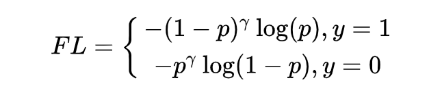
Taking binary classification as an example, cross-entropy is generally used as the model loss.
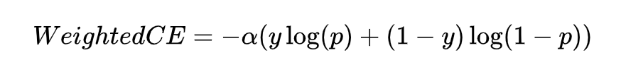
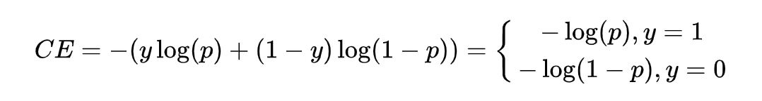 Where is the true label, is the predicted value, and based on this, a weighted cross-entropy is derived, using a hyperparameter to mitigate the aforementioned impact, represented by the following formula.
Next, let’s see how Focal Loss focuses on samples that are incorrectly predicted.
Based on the cross-entropy loss, when the predicted value of a positive sample is greater than 0.5, it needs to assign a small weight to its loss, making it have a small impact on the total loss. Conversely, when the predicted value is less than 0.5, a large weight is assigned to its loss. To satisfy the above requirements, when increases, should decrease, thus fulfilling the requirement.
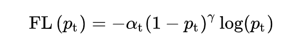
Therefore, adding an attention parameter, we obtain the Focal Loss for binary classification:
Adding a modulation factor, Focal Loss is extended to multi-class situations:
Where is the predicted value for class t, and in experiments, the best effect is achieved when .
The implementation of the code is also quite straightforward.
def __init__(self, num_class, alpha=None, gamma=2, reduction='mean'):
    super(MultiFocalLoss, self).__init__()
    self.gamma = gamma
    ......

    def forward(self, logit, target):
        alpha = self.alpha.to(logit.device)
        prob = F.softmax(logit, dim=1)

        ori_shp = target.shape
        target = target.view(-1, 1)

        prob = prob.gather(1, target).view(-1) + self.smooth  # avoid nan
        logpt = torch.log(prob)

        alpha_weight = alpha[target.squeeze().long()]
        loss = -alpha_weight * torch.pow(torch.sub(1.0, prob), self.gamma) * logpt

        if self.reduction == 'mean':
            loss = loss.mean()

        return loss
The Focal Loss above emphasizes learning from hard examples, but not all hard examples are worth focusing on; some hard examples may be outliers, which should not be emphasized by the model.
GHM (Gradient Harmonizing Mechanism) is a gradient harmonizing mechanism. The improvement ideas of GHM Loss have two points: 1) it allows the model to continue focusing on hard examples while preventing it from paying attention to outlier samples; 2) in Focal Loss, the values of are derived from experimental experience, but generally, hyperparameters influence each other and should be experimented together.
In Focal Loss, by adjusting the confidence level when the predicted value of positive samples is relatively small, a large loss value is given to make the model focus on such samples.Thus, GHM Loss builds on this by specifying a confidence range , specifically, when the predicted value of positive samples is relatively small, we need to see how small this is. If it is , such samples may be outliers and should not be attended to.
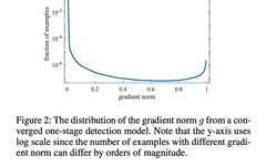
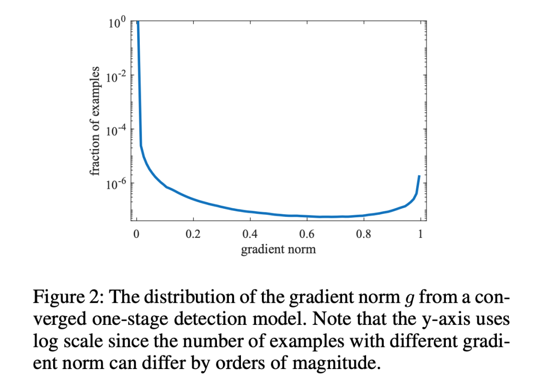
Therefore, GHM Loss first specifies agradient norm:
Where is the model’s predicted probability value, and is the ground-truth label value, taking binary classification as an example, the value is either 0 or 1. It can be seen that indicates the difficulty of detection, the larger the value, the more difficult the detection.
The idea of GHM Loss is to not focus on easily learned samples, nor on particularly difficult samples that are outliers. Thus, the problem becomes finding a variable to measure whether a sample belongs to either of these two categories.This variable needs to satisfy that when the value of is large, it should be small, thereby suppressing it, and when the value of is small, it should also be small, thus suppressing it. Therefore, the paper introduces gradient density:
It indicates the number of samples whose gradient norm falls within the range of 1 to N, and represents the length of the interval, thus the physical meaning of gradient density GD(g) is: the number of samples in the unit gradient norm section.
On this basis, there is also a premise that the number of samples with small and large values (i.e., easy-to-separate samples and hard-to-separate samples) far exceeds that of samples with intermediate values; only then can GD meet the requirements of the above variable.
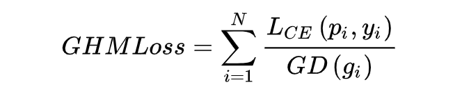
At this point, for each sample, multiplying the cross-entropy CE by the inverse of the gradient density of that sample gives GHM Loss.
Here is the logical code; the complete version can be found in the repository linked at the beginning and end of the article.
class GHM_Loss(nn.Module):
    def __init__(self, bins, alpha):
        super(GHM_Loss, self).__init__()
        self._bins = bins
        self._alpha = alpha
        self._last_bin_count = None

    def _g2bin(self, g):
        # split to n bins
        return torch.floor(g * (self._bins - 0.0001)).long()


    def forward(self, x, target):
        # compute value g
        g = torch.abs(self._custom_loss_grad(x, target)).detach()

        bin_idx = self._g2bin(g)

        bin_count = torch.zeros((self._bins))
        for i in range(self._bins):
            # 计算落入bins的梯度模长数量
            bin_count[i] = (bin_idx == i).sum().item()

        N = (x.size(0) * x.size(1))

        if self._last_bin_count is None:
            self._last_bin_count = bin_count
        else:
            bin_count = self._alpha * self._last_bin_count + (1 - self._alpha) * bin_count
            self._last_bin_count = bin_count

        nonempty_bins = (bin_count > 0).sum().item()

        gd = bin_count * nonempty_bins
        gd = torch.clamp(gd, min=0.0001)
        beta = N / gd  # 计算好样本的gd值

        # 借由binary_cross_entropy_with_logits,gd值当作参数传入
        return F.binary_cross_entropy_with_logits(x, target, weight=beta[bin_idx])
Dice Loss comes from the article V-Net, while DSC Loss is the Dice Loss for Data-imbalanced NLP Tasks proposed by Xiangnon Technology.
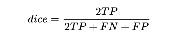
Following the logic above, let’s see how Dice Loss has evolved. Dice Loss is primarily derived from the dice coefficient, which is a measure function used to evaluate the similarity between two samples.
The definition is as follows: the range is from 0 to 1, with larger values indicating greater similarity. Let X be the set of all samples predicted as positive by the model, and Y be the set of all samples that are actually positive; the dice coefficient can be rewritten as:
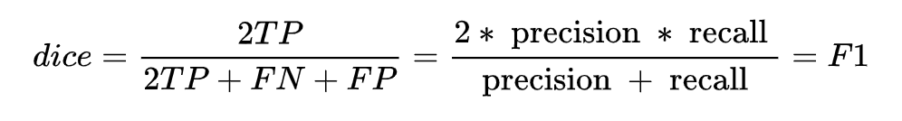
At the same time, combining the F1 metric calculation formula, we can derive:
By working through the calculations, we can find that the dice coefficient is equivalent to the F1 score; therefore, in essence, the dice loss directly optimizes the F1 metric.
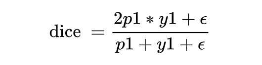
The above expression is discrete; we need to convert the DSC expression into a continuous version, which requires softening. For a single sample x, we can directly define its DSC:
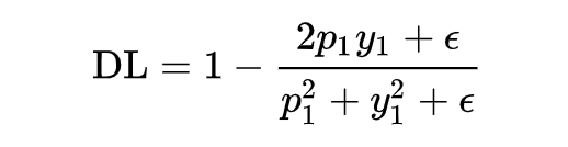
However, when the sample is a negative sample, y1=0, the loss becomes 0, so we need to add a smoothing term.
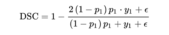
It has been mentioned that the dice coefficient is a measure function for the similarity of two samples. In the above expression, assuming that the positive sample p is larger, the dice value increases, indicating that the model’s prediction is more accurate, thus the loss value should be smaller. Therefore, the final form of the dice loss can be represented as follows:

To achieve the same functionality as focal loss, allowing dice loss to focus on incorrectly predicted samples, we can add a modulation factor , resulting in the self-adjusting DSC-Loss suitable for NLP tasks proposed by Xiangnon.
Having understood the principles, let’s look at the implementation of the code.
class DSCLoss(torch.nn.Module):

    def __init__(self, alpha: float = 1.0, smooth: float = 1.0, reduction: str = "mean"):
        super().__init__()
        self.alpha = alpha
        self.smooth = smooth
        self.reduction = reduction

    def forward(self, logits, targets):
        probs = torch.softmax(logits, dim=1)
        probs = torch.gather(probs, dim=1, index=targets.unsqueeze(1))

        probs_with_factor = ((1 - probs) ** self.alpha) * probs
        loss = 1 - (2 * probs_with_factor + self.smooth) / (probs_with_factor + 1 + self.smooth)

        if self.reduction == "mean":
            return loss.mean()
Conclusion
This article mainly discusses solutions to the class imbalance problem, which can be divided into data-level resampling and model loss improvements, such as focal loss and dice loss. Finally, based on practical experience, due to the varying distribution characteristics of different datasets, dice loss and GHM loss may exhibit some fluctuations and instability. When not wanting to experiment individually, focal loss and dice loss are recommended.
All the loss codes above are for logical reference; the complete code and related papers can be found at:
https://github.com/shuxinyin/NLP-Loss-Pytorch
Editor: Wang Jing
Proofreader: Yang Xuejun