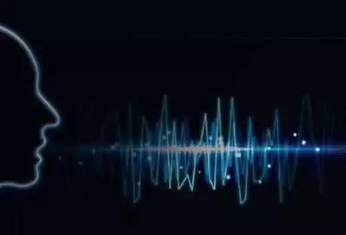
Speech is the most natural way for humans to interact. After the invention of computers, enabling machines to ‘understand’ human language, comprehend the intrinsic meaning within language, and provide correct responses became a pursuit for people. We all hope to have intelligent and advanced robotic assistants like those in science fiction movies, which can understand what we say during voice interactions. Speech recognition technology has turned this once-dreamed possibility into reality. Speech recognition is akin to the ‘hearing system of machines’, allowing machines to recognize and understand, converting speech signals into corresponding text or commands.

Speech recognition technology, also known as Automatic Speech Recognition (ASR), aims to convert the vocabulary content of human speech into computer-readable input, such as keystrokes, binary codes, or character sequences. Speech recognition is like the ‘hearing system of machines’; it allows machines to recognize and understand, transforming speech signals into corresponding text or commands.

Speech recognition is a broad interdisciplinary field closely related to acoustics, phonetics, linguistics, information theory, pattern recognition theory, and neurobiology. Speech recognition technology is gradually becoming a key technology in computer information processing.

Development of Speech Recognition Technology

Research on speech recognition technology began in the 1950s. In 1952, Bell Labs developed a recognition system for 10 isolated digits. Starting in the 1960s, researchers like Reddy at Carnegie Mellon University began studies on continuous speech recognition, but progress was slow during this period. In 1969, Pierce J of Bell Labs even compared speech recognition to something that would be impossible to achieve in recent years in an open letter.

In the 1980s, statistical model methods represented by the Hidden Markov Model (HMM) gradually dominated speech recognition research. The HMM model can effectively describe the short-term stationary characteristics of speech signals and integrate knowledge from acoustics, linguistics, and syntax into a unified framework. Subsequently, research and application of HMM became mainstream. For example, the first ‘speaker-independent continuous speech recognition system’ was the SPHINX system developed by Andrew Yao, who was studying at Carnegie Mellon University at the time. Its core framework is the GMM-HMM framework, where GMM (Gaussian Mixture Model) is used to model the observation probabilities of speech, and HMM models the temporal aspects of speech.

In the late 1980s, the predecessor of Deep Neural Networks (DNN), the Artificial Neural Network (ANN), also became a direction in speech recognition research. However, this shallow neural network generally did not perform as well as the GMM-HMM model in speech recognition tasks.

Starting in the 1990s, speech recognition saw a small resurgence in research and industrial applications, mainly due to the introduction of discriminative training criteria and model adaptation methods based on the GMM-HMM acoustic model. During this period, the Cambridge HTK open-source toolkit significantly lowered the barriers to speech recognition research. For nearly a decade afterward, progress in speech recognition research remained limited, with the overall performance of systems based on the GMM-HMM framework falling far short of practical levels, leading to a bottleneck in speech recognition research and application.

In 2006, Hinton proposed using Restricted Boltzmann Machines (RBM) to initialize the nodes of neural networks, leading to the development of Deep Belief Networks (DBN). DBNs addressed the issue of local optima in training deep neural networks, marking the official onset of the deep learning wave.

In 2009, Hinton and his student Mohamed D successfully applied DBNs to acoustic modeling in speech recognition, achieving success on small vocabulary continuous speech recognition databases like TIMIT.

In 2011, DNN achieved success in large vocabulary continuous speech recognition, marking the most significant breakthrough in speech recognition in nearly a decade. Since then, deep neural network-based modeling has officially replaced GMM-HMM as the mainstream approach in speech recognition modeling.

Basic Principles of Speech Recognition

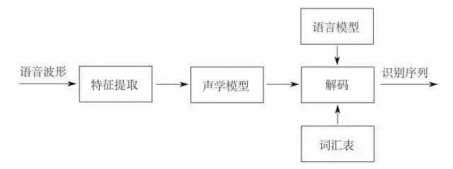
Speech recognition refers to the process of converting a segment of speech signal into corresponding text information. The system mainly consists of four components: feature extraction, acoustic models, language models, and dictionaries and decoding. To extract features more effectively, preprocessing of the collected sound signals is often required, including filtering and framing to extract the signals to be analyzed from the raw signals. Afterward, the feature extraction process converts the sound signal from the time domain to the frequency domain, providing suitable feature vectors for the acoustic model; the acoustic model then calculates the score of each feature vector based on its acoustic characteristics; the language model calculates the probability of the possible sequence of phrases corresponding to the sound signal based on linguistic theories; finally, the dictionary is used to decode the phrase sequence, resulting in the final possible text representation.

Acoustic Signal Preprocessing

The preprocessing of speech signals is crucial as a prerequisite and foundation for speech recognition. During the final template matching, the feature parameters of the input speech signal are compared with those in the template library. Therefore, it is essential to obtain feature parameters that represent the essential characteristics of the speech signal during the preprocessing phase to ensure high recognition rates.

First, the sound signal needs to be filtered and sampled to eliminate signals outside the range of human vocal frequencies and interference from 50Hz electrical currents. This process is generally achieved using a bandpass filter with set upper and lower cutoff frequencies, followed by quantization of the original discrete signals. Next, the high-frequency and low-frequency parts of the signal need to be smoothed to facilitate solving the spectrum under the same signal-to-noise ratio conditions, making analysis quicker and easier. The framing and windowing operation divides the original time-varying frequency domain signal into independent, frequency-stable segments by using different lengths of collection windows, primarily employing pre-emphasis techniques. Finally, endpoint detection is necessary to correctly identify the start and end points of the input speech signal, usually estimated using short-time energy (the amplitude of signal variation within the same frame) and short-time average zero-crossing rate (the number of times the sampled signal crosses zero within the same frame).

Acoustic Feature Extraction

After preprocessing the signals, the next step is the critical operation of feature extraction. Recognizing the original waveform does not yield good recognition results; instead, features extracted after frequency domain transformation are used for recognition, and the feature parameters used for speech recognition must meet the following criteria:

1. The feature parameters should adequately describe the fundamental characteristics of speech;

2. Minimize coupling between parameter components and compress the data;

3. The process of calculating feature parameters should be simplified, making algorithms more efficient. Parameters like fundamental frequency and formant values can serve as feature parameters characterizing speech.

Currently, the most commonly used feature parameters by mainstream research institutions include Linear Prediction Cepstral Coefficients (LPCC) and Mel-Frequency Cepstral Coefficients (MFCC). Both feature parameters operate on speech signals in the cepstral domain; the former takes a speech model as a starting point and uses LPC technology to compute cepstral coefficients, while the latter simulates the auditory model, using the output of a filter bank model as acoustic features, followed by discrete Fourier transformation (DFT).

The fundamental frequency refers to the vibration period of the vocal cords (fundamental frequency), which can effectively characterize speech signal features; thus, fundamental frequency detection has been a crucial research point since the early days of speech recognition research. Formants are regions of concentrated energy in speech signals, representing the physical characteristics of the vocal tract and being a primary determinant of speech quality, making them equally important feature parameters. Additionally, many researchers have begun applying methods from deep learning to feature extraction, achieving rapid progress.

Acoustic Models

Acoustic models are a vital component of speech recognition systems, and their ability to differentiate between different basic units directly impacts recognition results. Speech recognition is essentially a pattern recognition process, with the core of pattern recognition being classifiers and decision-making issues.

Typically, dynamic time warping (DTW) classifiers yield good recognition results in isolated word and small vocabulary recognition, offering quick recognition speeds and low system overhead, making them a successful matching algorithm in speech recognition. However, in large vocabulary and speaker-independent speech recognition, DTW performance declines sharply, whereas using Hidden Markov Models (HMM) for training shows significant improvement. In traditional speech recognition, continuous Gaussian mixture models (GMM) are generally used to characterize the state output density function, hence the GMM-HMM framework.

Moreover, with the development of deep learning, deep neural networks have been employed for acoustic modeling, forming the so-called DNN-HMM framework, which has also achieved good results in speech recognition.

Gaussian Mixture Models

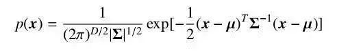
For a random vector x, if its joint probability density function conforms to formula 2-9, it is said to follow a Gaussian distribution, denoted as x ∼N(µ, Σ).

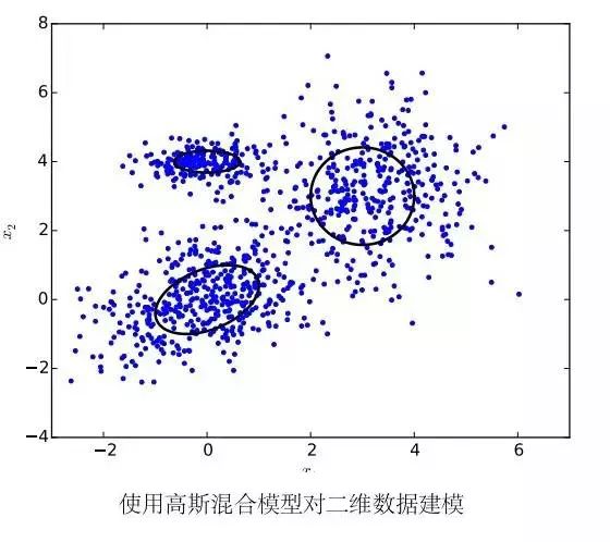
Here, µ represents the expected value of the distribution, and Σ is the covariance matrix of the distribution. Gaussian distributions have a strong ability to approximate real-world data and are easy to compute, making them widely used across various disciplines. However, many types of data are poorly described by a single Gaussian distribution. In such cases, we can use a mixture of multiple Gaussian distributions to model these data, with multiple components responsible for different underlying data sources. At this point, the random variable conforms to the density function.

Here, M represents the number of components, usually determined by the scale of the problem.

We refer to the model used to describe data following a mixture of Gaussian distributions as a Gaussian Mixture Model. Gaussian Mixture Models are widely used in the acoustic models of many speech recognition systems. Given that the dimensionality of vectors in speech recognition is relatively high, we usually assume that the covariance matrices Σm in the mixture of Gaussian distributions are diagonal matrices. This significantly reduces the number of parameters and improves computational efficiency.

Modeling short-term feature vectors using Gaussian Mixture Models has several advantages: first, Gaussian Mixture Models possess strong modeling capabilities; as long as the total number of components is sufficient, they can approximate a probability distribution function with arbitrary precision. Additionally, using the EM algorithm makes it easy for the model to converge on training data. To address issues like computational speed and overfitting, researchers have also developed parameter-tied GMMs and Subspace Gaussian Mixture Models (subspace GMMs). Besides using the EM algorithm for maximum likelihood estimation, we can also train Gaussian Mixture Models using discriminative error functions directly related to word or phoneme error rates, which can greatly enhance system performance. Therefore, until the emergence of deep neural networks in acoustic modeling, Gaussian Mixture Models remained the go-to choice for modeling short-term feature vectors.

However, Gaussian Mixture Models also have a significant drawback: they perform poorly in modeling data close to a nonlinear manifold in vector space. For instance, if some data are distributed on either side of a sphere and are very close to the surface, using an appropriate classification model may require only a few parameters to distinguish between the data on both sides of the sphere. However, if we use a Gaussian Mixture Model to depict their actual distribution, we would need many Gaussian distribution components to accurately characterize them. This drives us to seek a model that can more effectively utilize speech information for classification.

Hidden Markov Models

Now, let’s consider a discrete random sequence. If the transition probabilities conform to the Markov property, meaning that future states are independent of past states, it is called a Markov Chain. If the transition probabilities are time-invariant, it is termed a homogeneous Markov Chain. The output of a Markov Chain corresponds one-to-one with predefined states; for any given state, the output is observable and contains no randomness. If we extend the output so that each state of the Markov Chain outputs a probability distribution function, then the states of the Markov Chain cannot be directly observed and can only be inferred through other variables that conform to probability distributions influenced by state changes. We refer to models that use this hidden Markov sequence assumption to model data as Hidden Markov Models.

In the context of speech recognition systems, we use Hidden Markov Models to describe the sub-state transitions within a phoneme, addressing the correspondence between feature sequences and multiple basic speech units.

Using Hidden Markov Models in speech recognition tasks requires calculating the model’s likelihood over a segment of speech. During training, we need to use the Baum-Welch algorithm to learn the parameters of the Hidden Markov Model and perform maximum likelihood estimation (MLE). The Baum-Welch algorithm is a special case of the EM (Expectation-Maximization) algorithm, iteratively calculating the conditional expectations and maximizing conditional expectations using prior and posterior probability information.

Language Models

Language models primarily characterize the habitual ways in which human language is expressed, focusing on the intrinsic relationships between words in terms of their arrangement structure. During the decoding process of speech recognition, language models are referenced for word transitions, and a good language model can not only improve decoding efficiency but also enhance recognition rates to a certain extent. Language models are divided into rule-based models and statistical models; statistical language models use probabilistic methods to characterize the inherent statistical laws of language units, making them simple and practical in design while achieving good results, and they have been widely used in speech recognition, machine translation, sentiment recognition, and other fields.

The simplest yet most commonly used language model is the N-gram language model (N-gram LM). The N-gram language model assumes that the probability of the current word, given the context, only depends on the preceding N-1 words. Thus, the probability of the word sequence w1, . . . , wm can be approximated as

To obtain the probability of each word in the formula given the context, we need a sufficient amount of text in that language to estimate. We can directly calculate this probability using the proportion of word pairs containing the context within all word pairs, which is

For word pairs that do not appear in the text, we need to use smoothing methods for approximation, such as Good-Turing estimation or Kneser-Ney smoothing.

Decoding and Dictionary

The decoder is the core component of the recognition phase, decoding the speech using the trained model to obtain the most probable sequence of words or generating recognition lattices based on intermediate results for further processing by subsequent components. The core algorithm of the decoder is the dynamic programming algorithm, Viterbi. Due to the large decoding space, we typically use token passing methods with limited search widths in practical applications.

Traditional decoders dynamically generate decode graphs, such as the HVite and HDecode in the well-known speech recognition tool HTK (HMM Tool Kit). This implementation occupies less memory, but due to the complexity of each component, the overall system process is cumbersome, making it inconvenient to efficiently combine language models and acoustic models, and more challenging to scale. Currently, mainstream decoder implementations use pre-generated finite state transducers (FST) as pre-loaded static decode graphs to some extent. Here, we can construct the language model (G), vocabulary (L), context-related information (C), and Hidden Markov Model (H) into standard finite state transducers, and then combine them through standard finite state transducer operations to create a transducer from context-related phoneme sub-states to words. This implementation method uses some additional memory space but makes the instruction sequence of the decoder more organized, facilitating the construction of an efficient decoder. Additionally, we can pre-optimize the pre-constructed finite state transducers, merging and trimming unnecessary parts to make the search space more reasonable.

Working Principle of Speech Recognition Technology

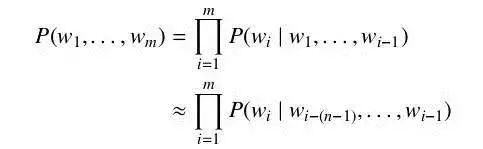
First, we know that sound is essentially a wave. Common formats like MP3 are compressed formats and must be converted to uncompressed pure waveform files for processing, such as Windows PCM files, commonly referred to as WAV files. Besides a file header, WAV files store the individual points of the sound waveform. The following figure shows an example of a waveform.

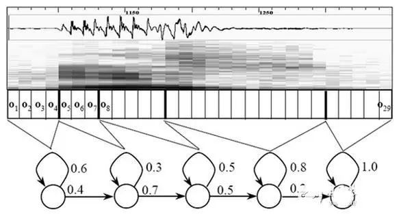
In the figure, each frame is 25 milliseconds long, with an overlap of 25-10=15 milliseconds between frames. This is referred to as framing with a frame length of 25ms and a frame shift of 10ms.

After framing, the speech is divided into many small segments. However, waveforms have almost no descriptive ability in the time domain, so they must be transformed. A common transformation method is to extract MFCC features, which convert each frame of waveform into a multidimensional vector based on the physiological characteristics of the human ear. This vector can be simply understood as containing the content information of that frame of speech. This process is called acoustic feature extraction.

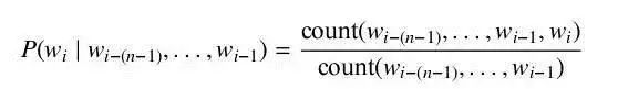
At this point, the sound becomes a matrix with 12 rows (assuming the acoustic features are 12-dimensional) and N columns, referred to as the observation sequence, where N is the total number of frames. The observation sequence is shown in the following figure, where each frame is represented by a 12-dimensional vector, and the color intensity of the blocks indicates the magnitude of the vector values.

Next, we need to introduce how to convert this matrix into text. First, let’s introduce two concepts:

Phoneme: The pronunciation of a word is composed of phonemes. For English, a commonly used phoneme set is a set of 39 phonemes from Carnegie Mellon University. In Chinese, the entire set of initials and finals is generally used as the phoneme set, and Chinese recognition also distinguishes between tones and non-tones, which will not be elaborated on here.

State: This can be understood as a more detailed speech unit than a phoneme. Typically, a phoneme is divided into three states.

How does speech recognition work? In reality, it is not mysterious at all; it is merely:

First, recognizing frames as states.

Second, combining states into phonemes.

Third, combining phonemes into words.

As shown in the figure below:

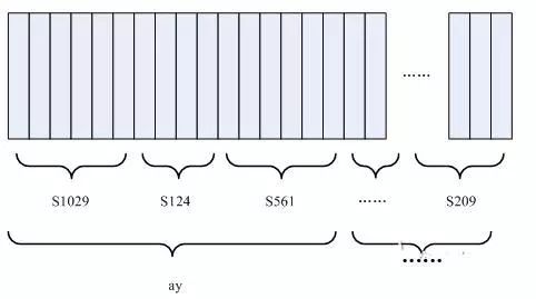
In the figure, each small vertical bar represents a frame; several frames correspond to a state, three states combine to form a phoneme, and several phonemes combine to form a word. In other words, as long as we know which state each frame of speech corresponds to, the result of speech recognition is determined.

So, how do we determine which state corresponds to each frame? A straightforward method is to look for the state with the highest probability for a given frame; thus, that frame is assigned to that state. For instance, in the following diagram, if the conditional probability for a frame is highest in state S3, we guess that this frame belongs to state S3.

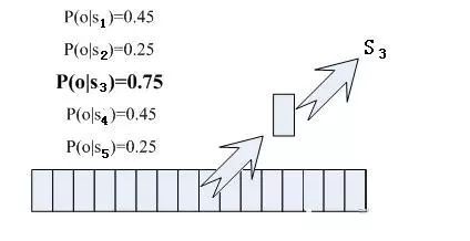
Where do these probabilities come from? There’s something called an ‘acoustic model’ that contains a large number of parameters; through these parameters, we can determine the probabilities corresponding to frames and states. The method of obtaining this large number of parameters is called ‘training’, which requires a vast amount of speech data.

However, this approach has a problem: each frame will receive a state number, leading to a chaotic array of state numbers for the entire speech. If the speech has 1000 frames, each frame corresponds to one state, and every three states combine to form a phoneme, we might end up with approximately 300 phonemes, but there aren’t actually that many phonemes in the speech. If we proceed this way, the resulting state numbers may not be able to combine into phonemes at all. In reality, it is reasonable for adjacent frames to share the same state, as each frame is quite short.

A common method to solve this problem is to use Hidden Markov Models (HMM). This concept may sound profound, but it is quite simple to use:

First, construct a state network.

Second, search for the path that best matches the sound from the state network.

This confines the results to a pre-set network, avoiding the issue mentioned earlier. Of course, this also brings a limitation; for instance, if your network only includes the state paths for ‘It is sunny today’ and ‘It is raining today’, no matter what is said, the recognized result will inevitably be one of those two sentences.

If you want to recognize arbitrary text, you need to build a sufficiently large network that encompasses all possible text paths. However, the larger the network, the more challenging it becomes to achieve a good recognition accuracy. Thus, one must reasonably choose the network size and structure according to the actual task requirements.

Building a state network involves expanding from a word-level network to a phoneme network and then to a state network. The speech recognition process is essentially about searching for the optimal path in the state network, where the probability of the speech corresponding to this path is maximized, known as ‘decoding’. The path search algorithm is a dynamic programming pruning algorithm known as the Viterbi algorithm, which is used to find the globally optimal path.

The cumulative probability mentioned here consists of three parts:

Observation probability: The probability corresponding to each frame and each state.

Transition probability: The probability of each state transitioning to itself or to the next state.

Language probability: The probability derived from the statistical laws of language.

The first two probabilities are obtained from the acoustic model, while the last probability is sourced from the language model. The language model is trained using a large corpus of text, leveraging the statistical patterns inherent in a language to help improve recognition accuracy. Language models are crucial; without them, when the state network is large, the recognized results may end up being a chaotic mix.

Thus, the basic process of speech recognition is completed, which is the working principle of speech recognition technology.

Workflow of Speech Recognition Technology

Generally speaking, a complete speech recognition system’s workflow can be divided into seven steps:

1. Analyze and process the speech signal, removing redundant information.

2. Extract key information impacting speech recognition and features that express language meaning.

3. Identify words based on the extracted feature information using minimal units.

4. Recognize words according to the grammar of different languages in sequence.

5. Use the preceding and following meanings as auxiliary recognition conditions to aid analysis and recognition.

6. Based on semantic analysis, segment key information and extract the recognized words, connecting them while adjusting sentence structure based on meaning.

7. Combine semantics to carefully analyze the interconnections of the context, making appropriate corrections to the currently processed sentences.

The principles of speech recognition can be summarized in three points:

1. The encoding of language information in speech signals is conducted according to the time variation of the amplitude spectrum;

2. Since speech can be read, i.e., acoustic signals can be represented by multiple distinguishable, discrete symbols without considering the content conveyed by the speaker;

3. Speech interaction is a cognitive process, so it must not be separated from grammar, semantics, and usage norms.

Preprocessing includes sampling of speech signals, overcoming aliasing filters, and removing noise effects caused by individual pronunciation differences and the environment. Repeated training involves having the speaker repeat the speech multiple times to eliminate redundant information from the original speech signal samples, retaining key information, and organizing the data according to certain rules to form a pattern library. Finally, pattern matching is the core part of the entire speech recognition system, judging the meaning of the input speech based on certain rules and calculating the similarity between the input features and the stored patterns.

Front-end processing first involves processing the raw speech signal, followed by feature extraction, eliminating noise and the effects of different speakers’ pronunciations, ensuring the processed signal can more completely reflect the essential characteristics of speech.

Source: Sensor Technology